A Survey on Theories and Applications for Self-Driving Cars Based on Deep Learning Methods

Abstract

Self-driving cars are a hot research topic in science and technology, which has a great influence on social and economic development. Deep learning is one of the current key areas in the field of artificial intelligence research. It has been widely applied in image processing, natural language understanding, and so on. In recent years, more and more deep learning-based solutions have been presented in the field of self-driving cars and have achieved outstanding results. This paper presents a review of recent research on theories and applications of deep learning for self-driving cars. This survey provides a detailed explanation of the developments of self-driving cars and summarizes the applications of deep learning methods in the field of self-driving cars. Then the main problems in self-driving cars and their solutions based on deep learning methods are analyzed, such as obstacle detection, scene recognition, lane detection, navigation and path planning. In addition, the details of some representative approaches for self-driving cars using deep learning methods are summarized. Finally, the future challenges in the applications of deep learning for self-driving cars are given out.

1. Introduction

Recently, the rapid development of artificial intelligence has greatly promoted the progress of unmanned driving, such as self-driving cars, unmanned aerial vehicles, and so on [1,2]. Among these unmanned driving technologies, self-driving cars have attracted more and more attention for their important economic effect [3]. However, there are lots of challenges in self-driving cars [4,5]. For example, the safety problem is the key technology that must be solved efficiently in self-driving cars, otherwise, it is impossible to allow self-driving cars on the road. Deep learning is an important part of machine learning and has been a hot topic recently [6,7]. Due to its excellent performances, it has been applied by scientists in the research and development of self-driving cars. More and more solutions based on deep learning for self-driving cars have been presented, including obstacle detection, scene recognition, lane detection, and so on.

This paper provides a survey on theories and applications of deep learning for self-driving cars. We introduce the theoretical foundation of the main deep learning methods used for self-driving cars. On this basis, we focus exclusively on the applications of deep learning for self-driving cars. Other relevant surveys in the field of deep learning and self-driving cars can be used as a supplement to this paper (see e.g., [1,6,8,9]).

The main contributions of this paper are summarized as follows. (1) A comprehensive analysis and review of the development of self-driving cars are presented. In addition, the challenges and limitations of current methods are enumerated. (2) A survey on the theoretical foundation of deep learning methods is given out, which focuses on the network structure. (3) An overview of the applications in self-driving cars based on deep learning is given out, and the details of some representative approaches are summarized. At last, some prospects of future studies in this field are discussed.

This paper is organized as follows: In Section 2, a general introduction to the development of self-driving cars is provided. A comprehensive analysis is given out on the development of the hardware and software technologies in this field. Section 3 introduces the theoretical background of some common deep learning methods used for self-driving cars. The main applications and some representative approaches based on deep learning methods in the field of self-driving cars are summarized in Section 4. Section 5 discusses the future research directions for the deep learning methods in self-driving cars. Finally, conclusions are given out in Section 6.

2. Development of Self-Driving Cars

The rapid development of the Internet economy and Artificial Intelligence (AI) has promoted the progress of self-driving cars. The market demand and economic value of self-driving cars are increasingly prominent [3]. At present, more and more enterprises and scientific research institutions have invested in this field. Google, Tesla, Apple, Nissan, Audi, General Motors, BMW, Ford, Honda, Toyota, Mercedes, Nvidia, and Volkswagen have participated in the research and development of self-driving cars [8].

Google is an Internet company, which is one of the leaders in self-driving cars, based on its solid foundation in artificial intelligence [10]. In June 2015, two Google self-driving cars were tested on the road (as shown in Figure 1a). So far, Google vehicles have accumulated more than 3.2 million km of tests, becoming the closest to the actual use. Another company that has made great progress in the field of self-driving cars is Tesla. Tesla was the first company to devote self-driving technology to production. Followed by the Tesla models series, its “auto-pilot” technology has made major breakthroughs in recent years. Although the tesla’s autopilot technology is only regarded as Level2 stage by the national highway traffic safety administration (NHTSA), as one of the most successful companies in autopilot system application by far, Tesla shows us that the car has basically realized automatic driving under certain conditions (see Figure 1b) [11].

In addition to the companies mentioned above, lots of Internet companies and car companies worldwide are also focusing on the self-driving car field recently. For example, in Sweden, Volvo and Autoliv established a joint company-Zenuity, which is committed to the security of self-driving cars [12]. In South Korea, Samsung received approval from the South Korean government to test its driverless cars on public roads in 2017. It should be noted that Samsung applied for the highest number of patents in the world in the field of self-driving cars from 2011 to 2017 [13]. In China, Baidu deep learning institute led the research project of self-driving cars in 2013. In 2014, Baidu established the automotive networking business division and successively launched CarLife, My-car, CoDriver and other products [14]. In 2016, Baidu held a strategic signing ceremony with Wuzhen Tourism, announcing that the unmanned driving at Level4 will be implemented in this scenic area (see Figure 2a). Other information technology (IT) companies in China also have intensively studied and made great progress in this field based on their technology in the field of artificial intelligence, such as Tencent, Alibaba, Huawei, and so on [15]. For example, Tencent has displayed the red flag Level3 self-driving car in cooperation with FAW (First Auto Work) (see Figure 2b).

According to the autonomous driving level, a car in Level0 to Level2 needs a driver to mainly monitor the environment. Advanced Driver Assistance Systems (ADAS) are intelligent systems that reside inside the vehicles categorized from Level0 to Level2 and help the driver in the process of driving [16,17]. The risks can be minimized based on the ADAS, such as the electronic stability control system and forward emergency braking system, by reducing driver errors, continuously alerting drivers, and controlling the vehicle if the driver is incompetent [18].

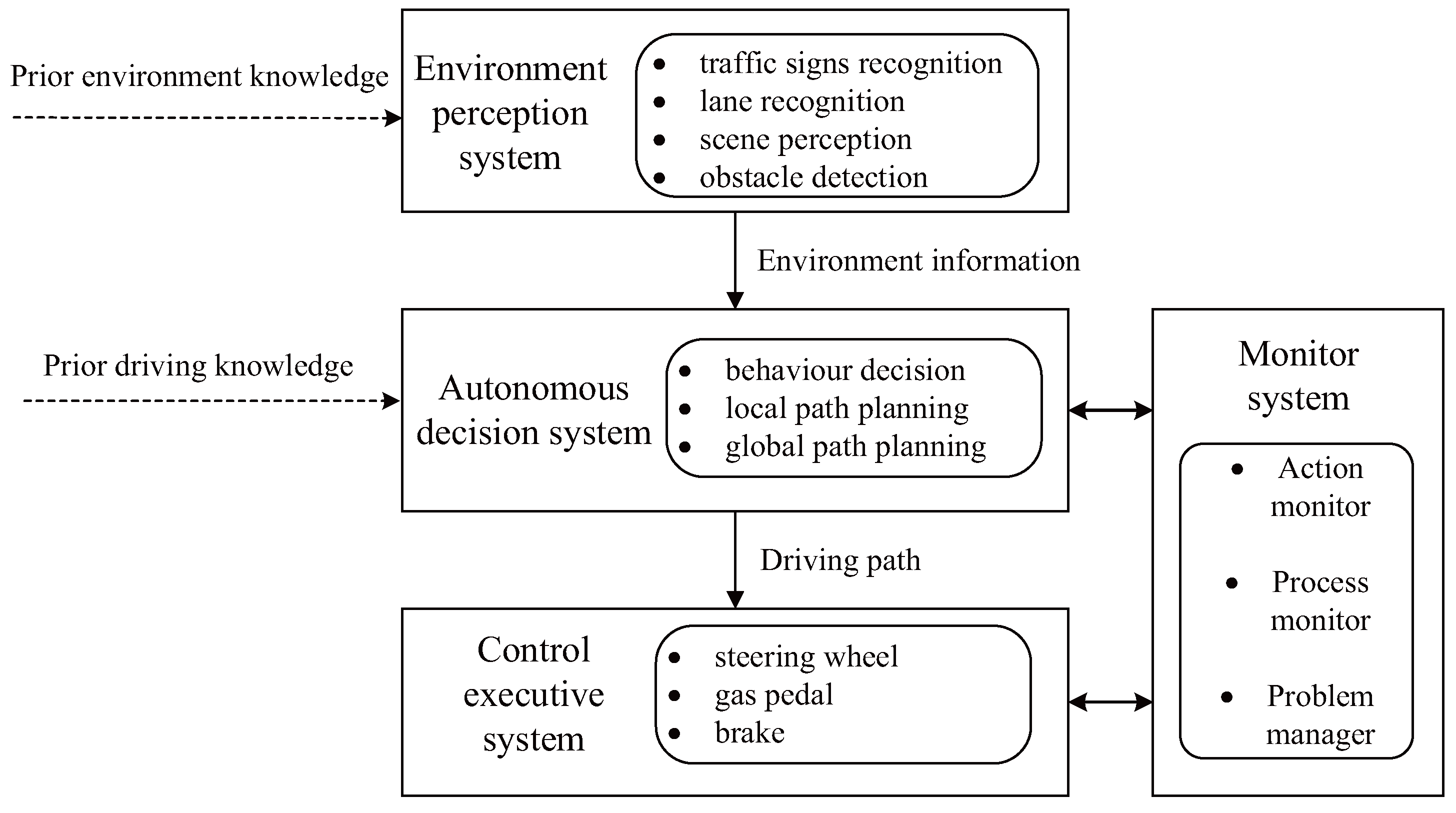
In this paper, we focus on self-driving cars which are categorized as level 3 or above. The overall technical framework of self-driving cars that are equipped with a Level3 or higher autonomy system can be divided into four parts, namely the driving environment perception system, the autonomous decision system, the control execution system and the monitor system [19]. The architecture of it is shown in Figure 3.

The environment perception system utilizes the prior knowledge of the environment to establish an environmental model including obstacles, road structures, and traffic signs through obtaining surrounding environmental information. The main function of the environment perception system is to realize functions like lane detection, traffic signal detection, and obstacle detection, by using some hardware devices such as cameras and laser radars.

The main function of the autonomous decision system is to make some decisions for the self-driving car, including obstacle avoidance, path planning, navigation, and so on. For example, in the path planning, the autonomous decision system plans a global path according to the current location and the target location firstly, then reasonably plans a local path for the self-driving car by combining the global path and the local environment information provided by the environment perception system.

The control execution system’s function is to execute the commands received from the autonomous decision system, such as braking, steering, and accelerating to complete the speed control and path-following control. The control execution system will perform some actions according to the situations of the environment directly sometimes, without any commands from the autonomous decision system, to deal with some emergencies, such as pedestrian avoidance.

The monitor system is responsible to check whether the car is making actual progress towards its goal and reacts with recovery actions when meeting problems like unexpected obstacles, faults, etc.

The self-driving car is a complex autonomous system, which requires the support of the theories and technologies. At the technical level, it is impossible to achieve such rapid development of the self-driving car without the rapid development of the hardware and software. There are various good hardware and soft platforms capable of rapid data analysis, as well as managing and understanding of self-driving cars [20]. For example, the NVIDIA DRIVE PX2 driverless car platform can perform 30 trillion deep learning operations per second and can achieve Level4 autopilot [21]. It supports 12-channel camera inputs, laser positioning, radar, and ultrasonic sensors, and includes two new-generation NVIDIA Tegra processors (see Figure 4). When it comes to softwares, Tensorflow is one of the main libraries for deep learning used in the field of self-driving cars [22].

At the theoretical level, some methods used in the robotic field can be applied in self-driving cars for the similarity between them, including path planning, environmental sensing, autonomous navigation and control, etc. [23,24]. Various artificial intelligence algorithms have been used in self-driving cars, such as fuzzy logic, neural network, and so on. Among these methods, deep learning methods have achieved great success in the self-driving field for their distinct advantages, such as high accuracy, strong robustness, and low cost. This paper will focus on the deep learning methods used in the field of self-driving cars.

Remark 1 (About the autonomous level of self-driving cars).

The NHTSA has adopted the level classification provided by the Society of Automotive Engineers, which ranges from Level 0 to Level 5 [25]. In this standard, Level 0 represents a vehicle without any autonomy. Level 1 has basic driving assistance such as adaptive cruise and emergency braking. Level 2 has partial autonomy while the driver needs to supervise the system and perform some tasks. At Level 3, the system has full autonomy under certain conditions, but the human operator is still required to take control if necessary. The vehicle at Level 4 is still a semi-autonomous system, which has higher automation than Level 3. Vehicles in Level 5 are fully autonomous in all conditions.

Remark 2 (About Tensorflow).

Tensorflow is a common deep learning platform that was created by Google. The design of Tensorflow is intended to simplify the construction of deep neural networks and speed up the learning process with a heterogeneous distributed computational environment [26]. Tensorflow provides lots of Application Programming Interface (API) libraries to build and train deep learning models, which can support Convolutional Neural Network (CNN), Recurrent Neural Network (RNN) and other deep neural network models.

3. Theoretical Background of Deep Learning Methods Used for Self-Driving Cars

During the last decade, deep learning has demonstrated to be an excellent technique in the field of AI. Deep learning methods have been used to solve various problems like image processing [27,28], speech recognition [29,30], and natural language processing [31,32]. As deep learning can learn robust and effective feature representation through layer-by-layer feature transformation of the original signal automatically, it has a good capability to cope with some challenges in the field of self-driving cars.

To introduce the applications of deep learning in the field of self-driving cars clearly, the theoretical background of four types of deep neural networks will be reviewed simply, which are the common deep learning methods applied to self-driving cars.

3.1. Convolutional Neural Network

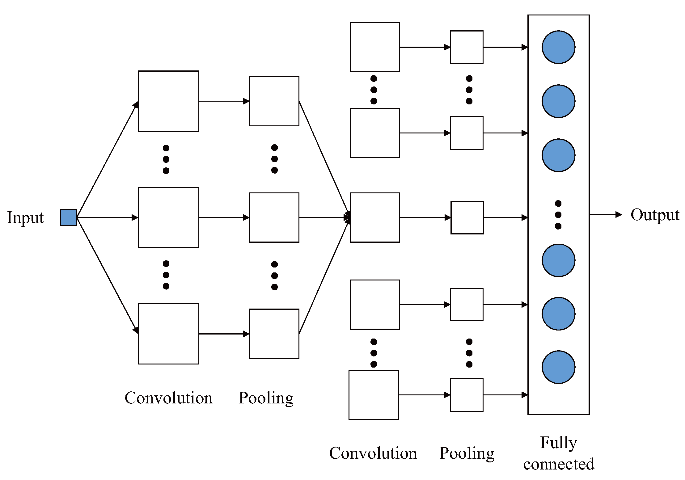
Convolutional Neural Network (CNN) is by far one of the most popular deep neural network architectures, usually consisting of an input layer, one or more convolution and pooling layers, a full connection layer, and an output layer at the top (see Figure 5).

Convolution layer is the core component of CNNs although the specific structures of CNNs may be different. The convolution kernel (i.e., filter matrix) is convolved with a local region of the input image, namely

$$y_j=\sum w_{ij}\ast x+b_j,$$

(1)

where the operator ∗ represents two-dimensional discrete convolution operation; w represents the filter matrix and b is the bias parameter; x is the input feature map and y represents the output of the feature map. The convolution kernel is generally initialized as a small matrix of $3\times 3$ or $5\times 5$. In the training process of the network, the convolution kernel will be constantly updated through learning and finally get a reasonable weight.

The output of the convolution operation is usually run by a nonlinear activation function. The activation function can help better to solve the linear inseparable problem. Functions such as Sigmoid, Tanh, and ReLU are usually used as activation functions, which are listed as follows:

$$\left\{\begin{array}{c}\mathrm{Sigmoid}:R=\frac{1}{1+e^{-y}}\hfill \\ \mathrm{Tanh}:R=\frac{e^y-e^{-y}}{e^y+e^{-y}}\hfill \\ \mathrm{ReLU}:R=max\left(0,y\right)\hfill \end{array}\right.$$

(2)

when the training gradient descends, ReLU is preferred as it has a faster convergence rate than traditional saturated nonlinear functions. In addition, the output of the convolution operation is modified by a pooling function. Mean-pooling and max-pooling are commonly used, which can keep more information about the background and the texture of the image respectively.

The success of the Convolutional Neural Network is due to its three important characteristics: local receptive fields, shared weights, and spatial sampling. The shared weight reduces the connection between the layers of the network and reduces the possibility of over-fitting. The pooling layer (i.e., subsampling layer) can reduce the dimension of the middle hidden layer and reduce the calculation amount of the next layer, and provide rotation invariance.

The CNN has yielded outstanding results in computer image and general image classification tasks recently. Because many self-driving cars technologies rely on image feature representation, they can be easily realized based on CNNs, such as obstacle detection, scene classification, and lane recognition.

3.2. Recurrent Neural Network

As the self-driving car functions depending on the information from the perception of constantly changing the surrounding environment, it is important to get a more complete representation of the environment by storing and tracking all the relevant information obtained in the past. Recurrent Neural Network (RNN) can be used to deal with this problem efficiently, which is mainly used to capture the time dynamics of video fragments.

Recurrent Neural Network maintains the memory of its hidden state for a period of time through a feedback loop and models the dependence relationship between the current input and the previous state [33]. A special type of RNN is Long Short–Term Memory (LSTM), which controls the input, output and memory state, to learn long-term dependencies [34] (see Figure 6).

In the RNN network, the current state of each loop unit is determined by the input at this moment and the previous state. Given the learning data input in sequence $X=\left\{x_1,x_2,\cdots x_t\right\}$, the hidden state at the time t is updated by:

$$H_t=\phi \left(U{X}_t+W{H}_{t-1}+b\right),$$

(3)

where the weight matrices U and W determine the importance given to the current input $X_t$ and to the previous state $H_{t-1}$ respectively; $\phi \left(·\right)$ is an activation function and b is the bias matrix. Then the output $O_t$ is calculated by:

$$O_t=V{H}_t+c,$$

(4)

where V is the weight matrix and c is the bias matrix.

3.3. Auto-Encoder (AE)

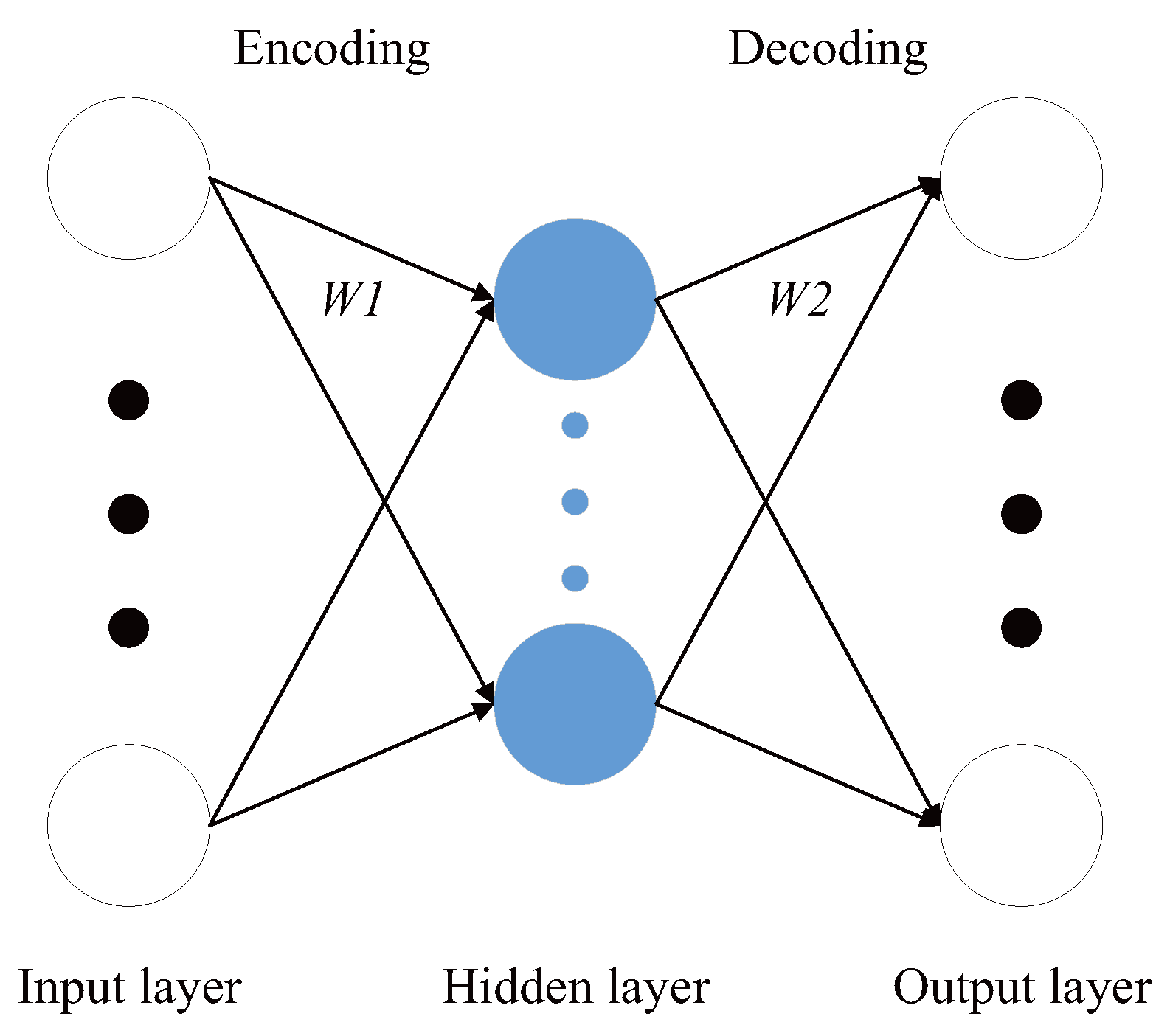
Large amounts of images obtained during the driving process lead to the explosive growth of dimensionalities, which will reduce the effectiveness of the calculation. To deal with this problem, Auto-Encoder (AE) is often applied, which is mainly used for dimensionality reduction and feature learning. AE is mainly composed of an encoder network, and a decoder network (see Figure 7).

As shown in Figure 7, the encoder is used to convert the high-dimensional original data into a low-dimensional vector representation, so that the compressed low-dimensional vector can retain the typical characteristics of the input data. The decoder is used to restore the original data. The training objective of AE is to minimize the error between the input and the output [35].

On the basis of the traditional AE, many improved methods are proposed to add some constraints on the hidden layer, forcing the hidden layer to express difference from the input. For example, the Convolutional Auto-Encoder (CAE) uses the convolution layer and pooling layer to replace the full connection layer of traditional AE, which can retain the spatial information of the two-dimensional signal. In the decoding process of CAE, deconvolution is used, which can be viewed as the inverse operation of convolution. By building a deconvolution network, the low resolution of feature representations can be mapped to the input resolution and the network generates accurate boundary localization with pixel-wise supervision [36].

3.4. Deep Reinforcement Learning (DRL)

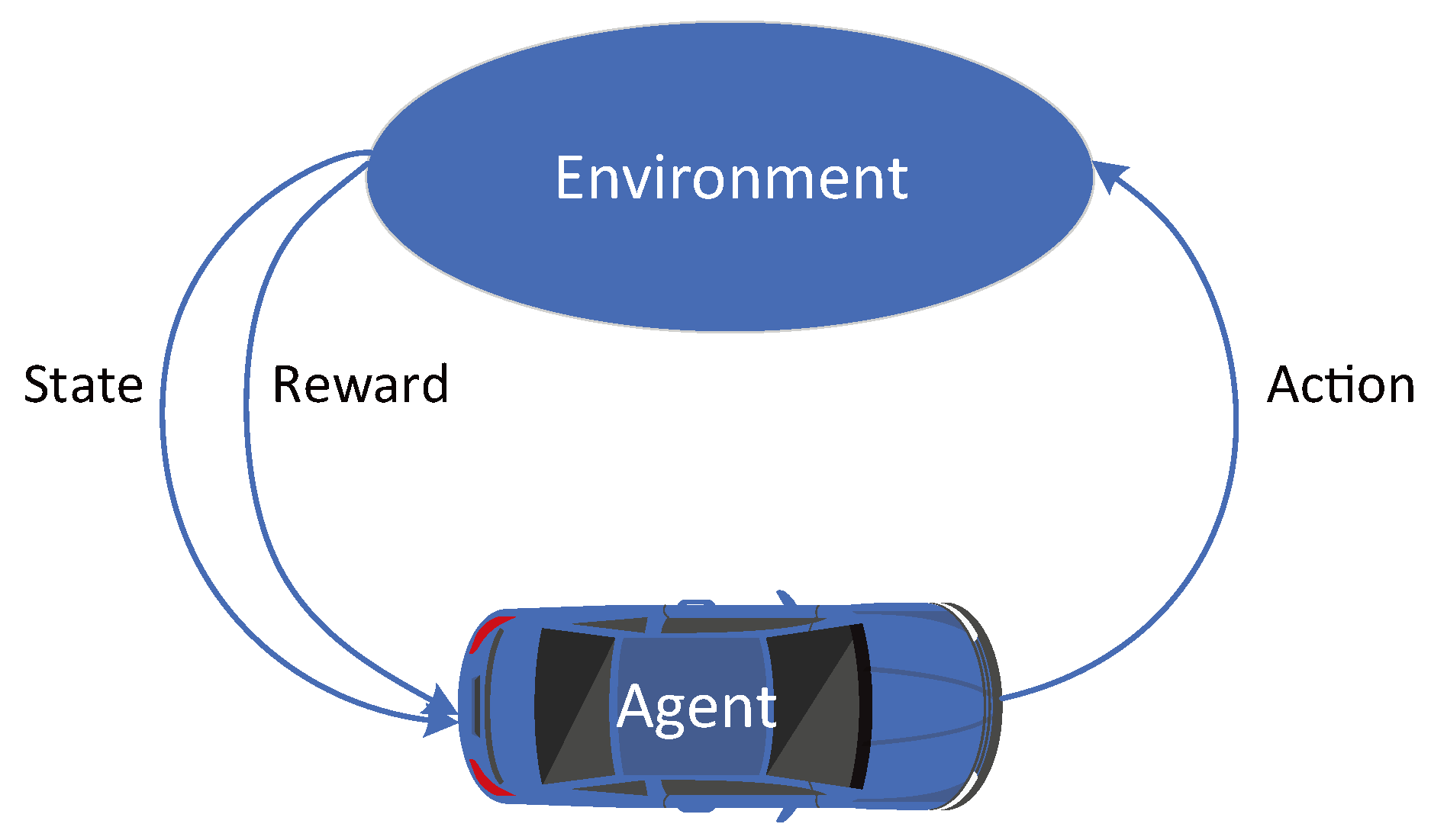
In recent years, the deep reinforcement learning method has been actively adopted to deal with various control problems in the unmanned vehicle field [37]. In reinforcement learning (RL), agents (like self-driving cars) can learn to modify their actions according to the rewards or punishments when interacting with environments (see Figure 8). The work process of RL can be described as the Markov Decision Process (MDP). In general, a MDP consists of a set of states $s\in S$, a set of actions $a\in A$, a reward function R and a transition model P [38].

A self-driving car (agent) perceives the current environment with state $s_t$ and performs an action $a_t$, then receives a reward $r\left(s_t,a_t\right)$ by the environment and transits to the next state $s_{t+1}$ according to the transition function $P\left(s_{t+1}\left|s_{t,}{a}_t\right.\right)$. The self-driving car is able to obtain a policy $\pi$, which maps every state $s_t$ to action $a_t$. The objective in RL is to maximize the accumulated discounted reward $R_t$, which is calculated by

$$R_t=\sum _{i=t}^T{\gamma }^{i-t}r\left(s_i,a_i\right),$$

(5)

where $\gamma$ is the discount factor that controls the importance of immediate and future rewards.

Q-learning is a model-free method of RL, where the action-value function $Q\left(s,a\right)=\underset{\pi }{max}\mathrm{E}[R_t\left|s_t,a_t,\pi ]\right.$ is used to represent the expectation of $R_t$ for every action-state pair $\left(s_t,a_t\right)$ and the function $\mathrm{E}[·]$ denotes the expected value of a random variable [39,40]. Q-learning approach is based on the optimization of the action-value function, which is calculated as follows:

$$Q^{*}\left(s_t,a_t\right)=\mathrm{E}\left[r\left(s_t,a_t\right)+\gamma \underset{a_{t+1}}{maxQ\left(s_{t+1},a_{t+1}\right)}\right],$$

(6)

where $Q^{*}$ is the optimal value of Q. The optimal policy ${\pi }^{*}$ is to maximize the value function, namely

$${\pi }^{*}=\underset{\pi }{argmax}{Q}^{*}\left(s,a\right).$$

(7)

Deep reinforcement learning (DRL) combines deep learning and reinforcement learning to solve the problem of capacity limitation and sample correlation. DRL has both the perceptive ability of deep learning and the decision-making ability of RL in a general form. DRL can learn a mapping from the original input to the action output [41]. One of the DRL methods is Deep Q-Network (DQN), which can utilize a deep neural network to map the relationships of actions and states, which is similar to the Q-learning method [42]. The DQN uses a CNN as the function approximator with weights $\theta$ as a Q-network, which is shown as follows:

$$y_i=Q_i^{*}\left(s_t,a_t\right)=\mathrm{E}\left[r\left(s_t,a_t\right)+\gamma \underset{a_{t+1}}{max}Q\left(s_{t+1},a_{t+1};{\theta }_{i-1}\right)\left|s_t,a_t\right.\right],$$

(8)

then the Q-network can be trained by updating the parameters ${\theta }_i$ in each iteration i by minimizing the mean-squared error as follows:

$$L_i\left({\theta }_i\right)=\mathrm{E}\left[{\left(y_i-Q\left(s_t,a_t;{\theta }_t\right)\right)}^2\right].$$

(9)

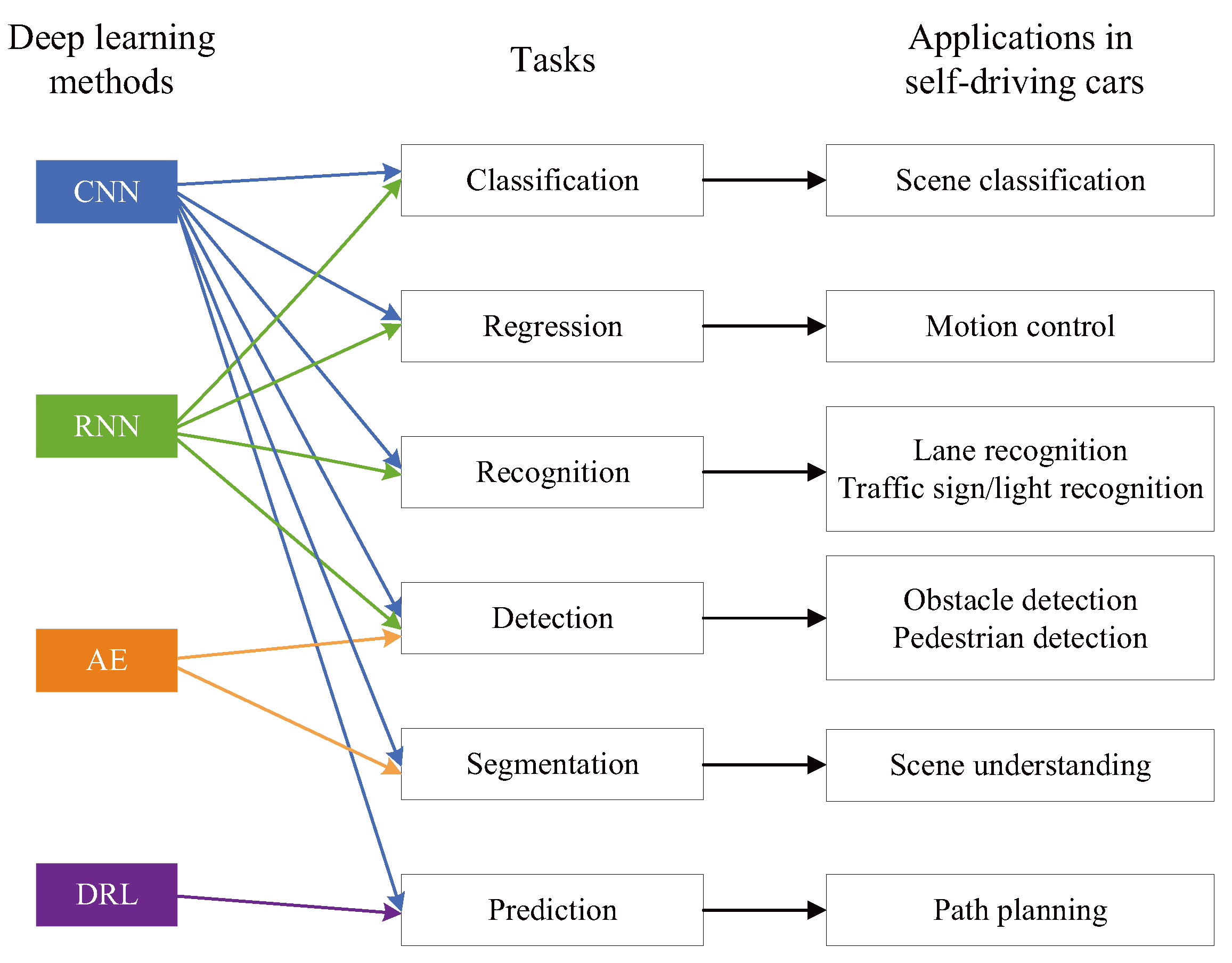
As introduced above, deep learning methods have many excellent characteristics that can meet the needs of self-driving cars. In this paper, the deep learning methods used in the field of self-driving cars can be classified based on their network structures, which are shown in Figure 9. The details of how the deep learning methods applied to self-driving cars will be clearly introduced in the next section.

4. Applications Overview of Deep Learning in the Field of Self-Driving Cars

As introduced in Section 3, deep learning has been used widely in the field of self-driving cars. In this section, the detailed applications based on various deep learning methods will be introduced. The main applications for self-driving cars based on deep learning summarized here are based on what the authors are most aware of, which can demonstrate the key issues and the latest advances in the field of self-driving cars. The main problems that must be addressed in self-driving cars include obstacle detection, scene recognition, lane recognition, and so on, which will be introduced in detail as follows.

4.1. Obstacle Detection

Obstacle detection technology is the most fundamental and core technical problem in self-driving systems, which is used to detect the target area that may block the normal driving of the vehicle, and guide the vehicle to avoid obstacles in time through the control system. In recent years, various sensors have been developed and equipped on self-driving cars to realize obstacle detection and recognition, such as the vision sensor, the ultrasonic sensor, the radar sensor, the lidar sensor, and so on [43,44]. Compared with detection technology based on other sensors, the vision sensor-based detection technology has many advantages, such as fast sampling speed, a large amount of information, and relatively low price. Obstacle detection technology based on vision sensors mainly includes a monocular vision and binocular vision [45].

The traditional monocular visual detection technology mainly relies on the manual design features to construct the model, and the quality of the model depends on the prior knowledge of the designer, so the recognition accuracy of this kind of algorithm is not high. The development of deep learning has revolutionized machine vision, and there are lots of research results in this field. For example, Mancini, et al. [46] proposed a CNN architecture, which can jointly finish the learning task for depth estimation and obstacle detection. Chen [47] presented a monocular vision-based algorithm. It can detect obstacles and identify obstacle-aware regions by implementing a deep encoder-decoder network. Parmar, et al. [48] proposed an improved CNNs based on the addition of a range estimation layer, which can accomplish obstacle detection, classification and ranking simultaneously.

The advantage of binocular vision over monocular vision is that 3D information of the scene can be directly obtained, and the geometric relationship between obstacles and road surface can be supplemented, so as to serve as the segmentation basis to realize obstacle detection. The flow chart of obstacle detection using binocular vision technology is shown in Figure 10. First, binocular images are acquired by the binocular camera, and a disparity map is obtained by the stereo matching algorithm. Then the calculation of the disparity map determines whether it is an obstacle point. Finally, the obstacle area is extracted.

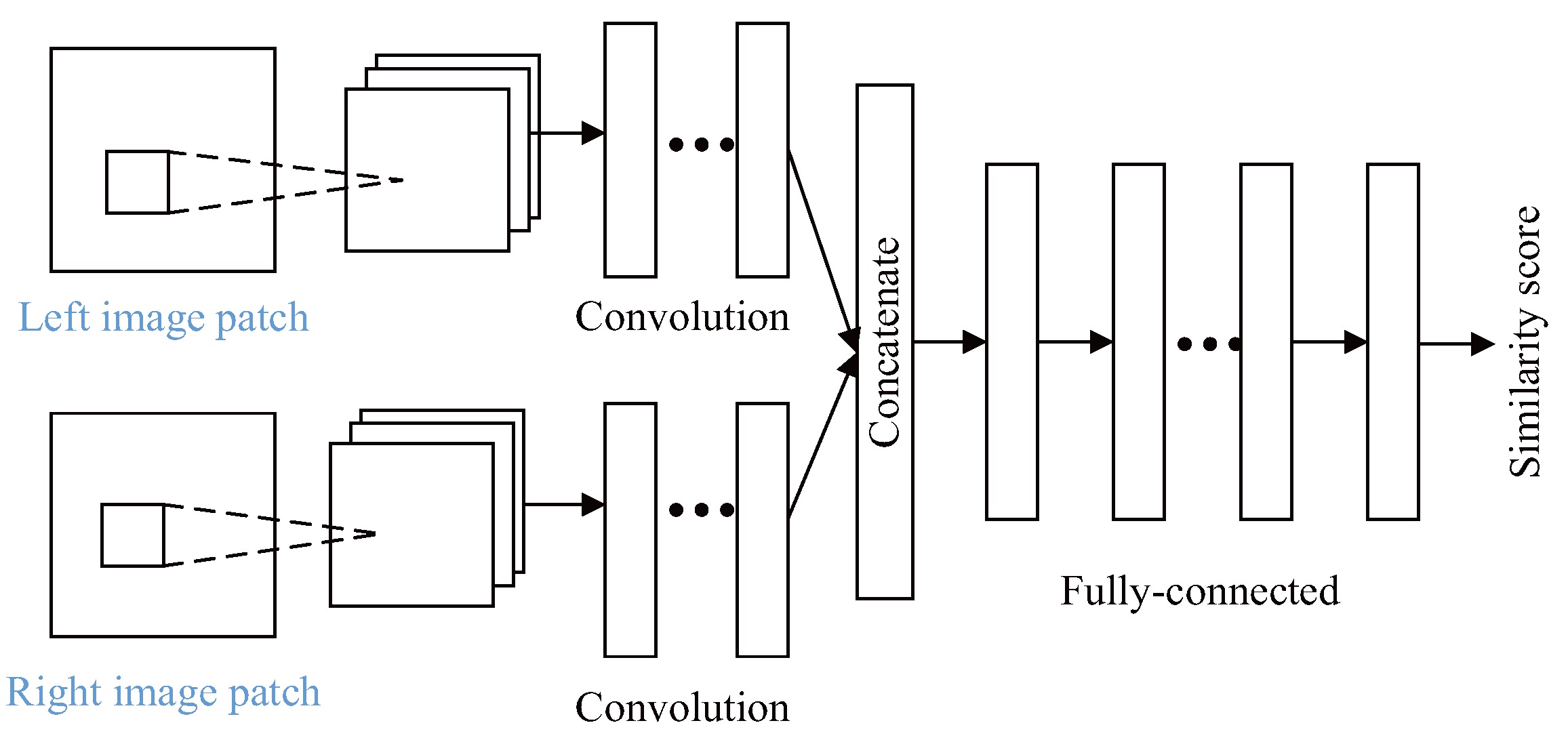
Typical stereo matching algorithms include the following four steps: matching cost computation, cost aggregation, disparity computation, and disparity refinement [49]. There are many research results on the binocular vision obstacle detection based on deep learning. For example, $\check{\mathrm{Z}}$bontar, et al. [50] designed a twin convolution structure MC-CNN (Matching Cost-Convolutional Neural network), where the CNN was applied to the image similarity measure and matching cost calculation. The structure of this MC-CNN is shown in Figure 11.

In the twin convolution structure of MC-CNN, there are many convolutional layers in the networks. Each layer is followed with a rectified linear unit. Then the obtained two vectors are connected in series and propagated by the fully-connected layers. At last, a single number is produced by the last fully-connected layer. This number denotes the similarity rate between the input patches. In the method of [50], the matching cost is directly initialized from the output of the network:

$$C_{\mathrm{CNN}}\left(\mathbf{p},d\right)=-s\left(<P^L\left(\mathbf{p}\right),P^R\left(\mathbf{p}-d\right)>\right),$$

(10)

where $s\left(·\right)$ is the output function; $P^L\left(\mathbf{p}\right)$ and $P^R\left(\mathbf{p}-d\right)$ are the input patches from the left image and the right image respectively; $\mathbf{p}$ denotes the position $(x,y)$, and d is the correct disparity at this position.

The cost aggregation process of stereo matching in MC-CNN is as follows:

$$\begin{array}{c}{C}_{\mathrm{CBCA}}^0=C_{\mathrm{CNN}}\left(\mathbf{p},d\right)\hfill \\ C_{\mathrm{CBCA}}^i=\frac{1}{\left|U_d\left(\mathbf{p}\right)\right|}{\displaystyle \sum _{\mathbf{q}\in U_d\left(\mathbf{p}\right)}}{C}_{\mathrm{CBCA}}^{i-1}\left(\mathbf{q},d\right),\hfill \end{array}$$

(11)

where, $U_d\left(\mathbf{p}\right)$ denotes the combined support region for $\mathbf{p}$; i is the number of iterations.

The final matching cost $C_{\mathrm{SGM}}$ is defined as the average across of the four directions $\mathbf{r}$, namely:

$$C_{\mathrm{SGM}}\left(\mathbf{p},d\right)=\frac{1}{4}\sum _{\mathbf{r}}{C}_{\mathbf{r}}\left(\mathbf{p},d\right)$$

(12)

$$C_{\mathbf{r}}\left(\mathbf{p},d\right)=C_{\mathrm{CBCA}}^4\left(\mathbf{p},d\right)-\underset{k}{min}{C}_{\mathbf{r}}\left(\mathbf{p}-\mathbf{r},k\right)+min\left\{\begin{array}{c}{C}_{\mathbf{r}}\left(\mathbf{p}-\mathbf{r},d\right),\hfill \\ C_{\mathbf{r}}\left(\mathbf{p}-\mathbf{r},d-1\right)+P_1,\hfill \\ C_{\mathbf{r}}\left(\mathbf{p}-\mathbf{r},d+1\right)+P_1,\hfill \\ \underset{k}{min}{C}_{\mathbf{r}}\left(\mathbf{p}-\mathbf{r},k\right)+P_2\hfill \end{array}\right\},$$

(13)

where $P_1$ and $P_2$ are the penalty parameters. Then the disparity image D is calculated by finding the disparity d that minimizes $C\left(\mathbf{p},d\right)$, which is as follows:

$$D\left(\mathbf{p}\right)=\underset{d}{argmin}C\left(\mathbf{p},d\right).$$

(14)

After the disparity is calculated, the obstacle area can be detected, which makes it possible to detect the obstacle in the self-driving car. The experiment examples of disparity results using MC-CNN are shown in Figure 12.

The solution of the stereo matching algorithm lays a solid foundation for obstacle determination. There are other methods based on deep learning used in the obstacle detection for self-driving cars. For example, Nguyen, et al. [51] presented a network structure, which is constructed by a wide context learning network and stacked encoder-decoder 2D CNNs. Zhang, et al. [52] proposed an end-to-end multidimensional residual dense attention network, which focuses on more comprehensive pixel-level feature extraction. The network includes a two-dimensional residual dense attention network for feature extraction and a three-dimensional convolutional attention network for matching. Kendall, et al. [53] presented a deep learning network for regressing the disparity of a pair of stereo images, where the context is incorporated directly from the data employing 3D convolutional network. Dairi, et al. [54], proposed a method where a deep-stacked auto-encoders (DSA) model is used. In this DSA model, the greedy learning features are combined with the dimensionality reduction capacity. In addition, an unsupervised k-nearest neighbor algorithm is employed to detect the obstacles.

A summary of the deep-learning-based obstacle detection algorithms is illustrated in

Table 1. A summary of the deep learning method-based obstacle detection algorithms.

Category	Reference	Method	Remarks	Performances
Monocular vision	Mancini, et al. (2015) [46]	CNN	The input of the proposed network is an RGB image and the features are extracted by the VGG19 module. Then these features are used to obtain the dense depth maps and obstacles bounding boxes based on CNNs.	Recall of 90.85% on UnrealDataset dataset.
	Parmar, et al. (2019) [48]	CNN	The range of the object in meters and class labels for each detected object are produced based on the proposed feed-forward CNN.	mAP of 96.92% on KITTI dataset.
	Mancini, et al. (2016) [55]	FCN	A fully convolutional network (FCN) is proposed, which is used to obtain depth estimation based on both images and optical flows.	RMSE of 6.863 on KITTI dataset.
	Jia, et al. (2016) [56]	CNN and DBN	The local information of a candidate block is generalized by CNN, and the global information of the whole image is generalized by DBN. Then all the features are transferred to the final classifier together for obstacle detection.	Block accuracy of 90.64% on KITTI dataset.
Binocular vision	$\check{\mathrm{Z}}$bontar, et al. (2016) [50]	2D-CNN	A CNN architecture is presented for measuring the similarity of image patches, which is used to deal with the problem of stereo matching.	Misclassified pixels error of 2.43% on KITTI dataset.
	Nguyen, et al. (2019) [51]	2D-CNN	A wide context learning network is used to extract global context information. Then a stacked encoder-decoder 2D CNNs performs contextual aggregation followed by a regression step to predict the disparity map.	2PE of 4.35%, 3PE of 2.74% on KITTI dataset.
	Zhang, et al. (2019) [52]	3D-CNN	There are two parts in the proposed network, namely the 2D residual dense attention net and the 3D convolutional attention net. They are used for feature extraction and matching respectively.	2PE of 3.21%, 3PE of 2.09% on KITTI dataset.
	Kendall, et al. (2017) [53]	3D-CNN	The proposed method learns context in the disparity cost volume using 3-D convolutions and regresses sub-pixel disparity values from the disparity cost volume using a soft Argmin function.	2PE of 3.46%, 3PE of 2.30% on KITTI dataset.
	Dairi, et al. (2018) [54]	SAE	A deep stacked auto-encoders (SAE) model and an unsupervised k-nearest neighbor algorithm are used to detect the obstacles.	AUC of 0.91 on MSVUD and DUSD datasets.
	Zhong, et al. (2018) [57]	RNN	The input of the proposed RNN is a continuous stereo video. Then, a depth-map at each frame is predicted directly. There is no pre-training process, and no need of ground-truth disparity maps in the proposed method.	RMSE of 4.451 on KITTI dataset.
	Jie, et al. (2018) [58]	RNN	A left-right comparative recurrent model is proposed to perform left-right consistency checking jointly with disparity estimation.	Error rates of all the pixels of 3.03% on KITTI dataset.

Note: MAE means the mean absolute error; mAP means the mean average precision; RMSE means the root mean square error; 2PE means the 2-pixel-error for all pixels; 3PE means the 3-pixel-error for all pixels; and AUC means the area under the receiver operating characteristic curve.

, where the main methods used in the obstacle detection are given out and the corresponding references are also listed.

4.2. Scene Classification and Understanding

The classification and understanding of autonomous driving scenes refer to judge the current traffic scene and environment information of the vehicle. It realizes the distinction among different scenes relying on the record of visual environment data around the vehicle with an on-board camera. There are some differences between the scene classification and understanding. Scene classification outputs holistic scene categories by integrating information of a whole image including local objects, global structure and their relationships. Scene understanding partitions meaningful regions in a scene image and then labels these regions with different semantic classes. However, the distinction between the scene classification and scene understanding is not strict. They both belong to the scene recognition. Since the self-driving system relies on the results of environmental perception to make driving behavior decisions, the output results of scene recognition will have a profound and huge impact on the driving behavior of self-driving cars.

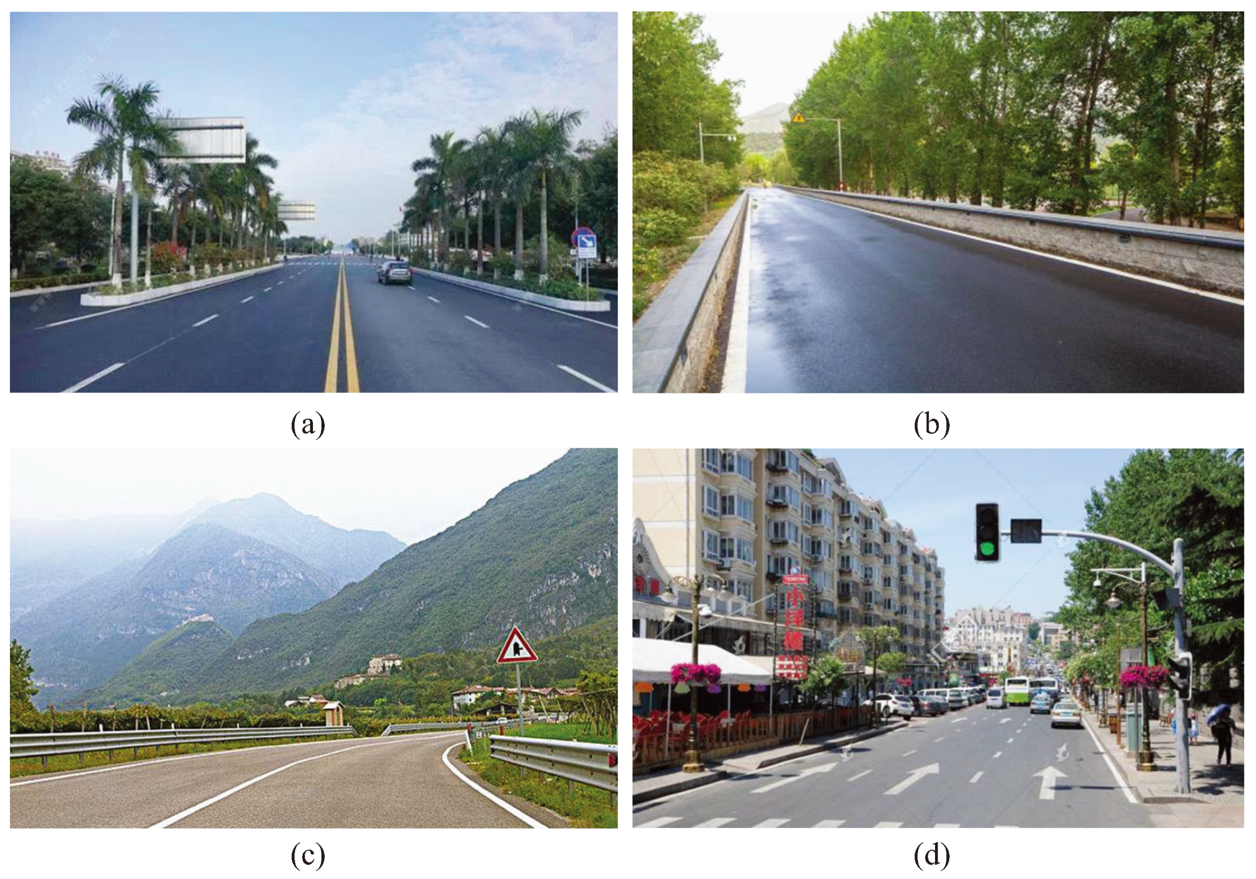
At present, great progress has been made in the recognition of driverless scenes, but there is still a lot of work to be done for self-driving cars to realize safe and autonomous driving in the complex traffic environment in real life. The instantaneity, robustness, and accuracy of road scene recognition are affected by multiple factors such as light variation, complex road environment and severe weather (as shown in Figure 13). Therefore, it is urgent to develop more mature and stable algorithms. Common outdoor scenes for the self-driving car include expressway, street, urban area, suburb, mountain, school, coast, etc (as shown in Figure 14) [59]. In order to achieve a higher level of intelligent driving, autonomous cars should know high-level semantic information in their places to make driving strategy and path planning decisions wisely. For example, cars should slow down near schools, pay attention to the use of anti-slippery mode/function during rain and snow and keep high speed through the highway, and so on.

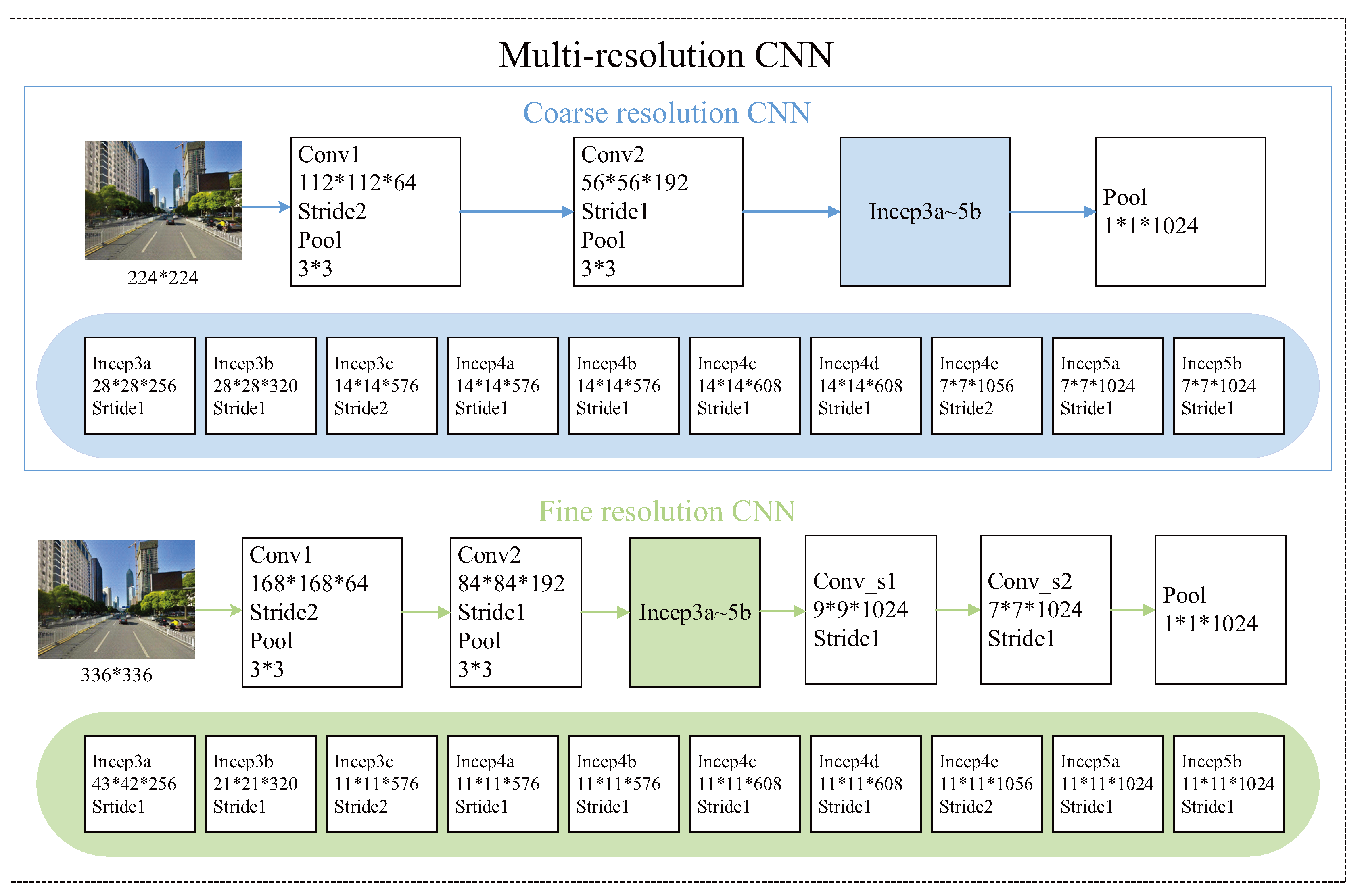
Deep learning shows obvious advantages in scene recognition. In recent years, the theoretical research and application of deep networks in scene recognition are also rich. For example, Wang, et al. [60] proposed a multi-resolution CNN network model, which won the first prize in the LSUN competition that year. This model includes coarse resolution CNNs and fine resolution CNNs, which are used to capture the visual structures at a large scale and a relatively smaller scale respectively. The architecture used in [60] takes two different resolution images as input (see Figure 15), so that it can be used for the scene understanding with different scales.

In the multi-resolution CNN in Figure 15, the coarse resolution architecture starts from two convolution layers and the max-pooling layer which converts a $224\times 224$ input image into a $28\times 28$ feature maps. The subsequent ten inception layers fast process the small size of feature maps. Because the coarse resolution CNNs focus on the global arrangements or objects at a larger scale, they capture visual appearance and structure at a relatively coarse resolution. The fine resolution CNNs use the $336\times 336$ image region as input. Three extra convolutional layers are added on top of the inception layer. The purpose of this structure is to capture the visual content in a finer resolution and enhance local detailed information.

In addition, the authors in [60] proposed a knowledge-based disambiguation method to deal with the problem of label ambiguity. Firstly, the knowledge of extra networks is exploited to provide supervised information for each image. Then the knowledge is used to guide the training process of the CNN networks. In the training process, the CNN networks can predict the hard labels (the ground-truth scene labels) and the soft labels (the predicted scene labels) simultaneously. The objective function used in [60] is as follows:

$$l\left(D\right)=-\left(\sum _{{\mathbf{I}}_i\in D}\sum _{k=1}^{K_1}\prod \left(y_i=k\right)log{p}_{i,k}+\lambda \sum _{{\mathbf{I}}_i\in D}\sum _{k=1}^{K_2}{q}_{i,k}log{f}_{i,k}\right),$$

(15)

where ${\mathbf{I}}_i$ denotes the i-th image in the training dataset D; $y_i$ and $p_i$ are the hard label (with $K_1$ dimension) and the soft label (with $K_2$ dimension) respectively; $f_i$ is the soft code produced by an extra knowledge network; $q_i$ is the predicted soft code of ${\mathbf{I}}_i$; and $\lambda$ is a balancing parameter.

The results of experiments on different datasets based on the proposed method in [60] are listed in

Table 2. The classification error on different datasets based on multi-resolution CNN in [60].

Method	ImageNet-1k	Places205	Places365	Places401
	(Top1/Top5)	(Top1/Top5)	(Top1/Top5)	(Top1/Top5)
Two-Resolution CNN	21.8%/6.0%	36.4%/10.4%	42.8%/13.2%	47.4%/16.3%

, which shows that the multi-resolution learning framework can improve the generalization ability by the knowledge obtained from extra networks. Furthermore, this framework can reduce the over-fitting during the training process.

In addition to the above multi-resolution CNN method, there are lots of research results in scene recognition based on deep learning methods. In terms of scene classification, Chen et al. [59] proposed a road scene recognition method based on a multi-label neural network. This network architecture integrates different classification modes into a cost function for training. Tang et al. [61], employed the GoogLeNet model for scene recognition, which is divided into three parts of layers from bottom to top and the output features from each of the three parts are fused to generate the final decision for scene recognition. When it comes to scene understanding, Fu et al. [36] presented a contextual deconvolution network embedding channel contextual module and spatial contextual module. The decoder network uses hierarchical supervision for multi-level feature maps to improve the representation of the scene semantic information. Byeon et al. [62] proposed a 2D-LSTM network to learn surrounding context information and model spatial dependencies of scene labels. The final layer outputs the class probabilities of each image patch.

A summary of the deep learning method-based scene recognition algorithms is illustrated in

Table 3. A summary of the deep learning method-based scene recognition algorithms.

Structure	Reference	Method	Remarks	Performances
GoogLeNet	Chen et al. (2019) [59]	CNN	A multi-label neural network is proposed for road scene recognition, where single and multiple class classification modes are incorporated into a multi-level cost function for training with imbalanced categories.	mAP of 83.1% on their own dataset.
GoogLeNet	Tang et al. (2017) [61]	CNN	GoogLeNet is partitioned into three parts, which are used to extract the features. Then these features are fused for the final recognition based on the product rule.	Accuracy of 92.90% on Scenel5 dataset.
ResNet	Zhang et al. (2019) [63]	CNN	The separate predictions are carried out based on the features obtained from multiple levels of the network. Then the final prediction is made by the ensemble learning within the network.	Top5 accuracy of 98.7% on UMC dataset.
ResNet	Liu, et al. (2019) [64]	CNN	A transfer learning model based on the ResNet is proposed, where the multi-layer feature fusion is utilized. The interlayer discriminating features are fused for classification by Softmax regression.	Accuracy of 94.05% on MIT67 dataset.
VGGNet	Cheng, et al. (2018) [65]	CNN	The correlations of object configurations among different scenes are exploited through the co-occurrence pattern of all objects across scenes, and then the representative and discriminative objects in the scene can be chosen.	Accuracy of 94.37% on Scene15 dataset.
Bn-Inception	Wang, et al. (2017) [60]	CNN	The proposed multi-resolution CNN architecture is composed of coarse resolution CNNs and fine resolution CNNs, which can capture visual content and structure at multiple levels.	Top5 error of 13.2% on Place365 dataset.
2D-LSTM	Byeon et al. (2015) [62]	RNN	In this approach, segmentation, classification, and context integration are all carried out by 2D LSTM RNNs, and the texture and spatial model parameters can be learned within a single model.	Pixel accuracy of 78.56% on Stanford Background dataset.
DenseNet	Fu et al. (2020) [36]	CAE	A contextual deconvolution network is proposed by embedding two types of contextual modules. The channel and the spatial contextual module utilize global and local features respectively.	Mean IoU of 80.5% on Cityscapes dataset.
CNN and RNN	Sun et al. (2019) [66]	Hybrid network	Deep features are extracted from the information of object semantics, global appearance, and contextual appearance. Then these features are fused for scene recognition based on a comprehensive representation.	Accuracy of 89.51% on MIT67 dataset.

Note: IoU means intersection over union.

, where the network structures of the corresponding methods are given out.

4.3. Lane Recognition

Lane detection is an important function of self-driving cars. Stable and accurate lane detection is the foundation of deviation warning, collision prevention, path planning, and other tasks. At present, there is no uniform definition for the baseline of lane detection, including the formation as lines, point sets or instances of lanes. So the lane detection methods discussed in this paper are not limited to a specific type of lane detection method. The traditional lane detection method uses the image processing algorithm, including the extraction of the possible lane areas, edge enhancement, extraction of the lane line feature and the lane. However, traditional image processing methods have higher demands to experience and are more sensitive to the interference of light, shade, and other external factors, which lead to a decrease in the adaptability and accuracy of the algorithms.

To deal with the disadvantages of the traditional image processing methods in lane detection, many scholars have applied deep learning to lane recognition. For example, John et al. [67] proposed a lane detection algorithm, where the semantic road lane is estimated using the regression and classification framework based on the extra tree. The input of this framework is extracted from the deconvolutional network. The training and testing process of the method proposed in [67] is shown in Figure 16.

As shown in Figure 16, in the training phase of the method in [67], Stage A is used to fine-tune the deconvolution network. The input of the deconvolution network is the combination of the hue, saturation, and depth (HSD). This deconvolution network is trained to extract the features of the road scene. Stage B is used to train the extra trees-based classifier for modeling the relationship between the road scene and the labels. Then this classifier is used to predict the scene labels based on the color and depth features of the road scenes. In Stage C, for each road scene label, a separate extra tree regressor is trained using the image-based deep features and the lane marker locations annotated manually. This extra tree regressor can be used to predict the lane marker position.

In the testing phase of the method in [67] (see Figure 16), the trained deconvolution network is used to predict the road surface and output the features of the road surface. Then, these features are input to the classifier model to get the scene label. At last, the estimated scene labels and the road features are input to the corresponding regression model, to predict the lane locations and the semantic information. Results of the algorithm proposed in [67] are shown in Figure 17.

In order to deal with complex noises and scenes in the lane detection for self-driving cars, lots of methods based on deep learning have been proposed. For example, Xiao, et al. [68] proposed an accurate and fast deep CNN, which combined self-attention and channel attention in lane marking detection. Kim, et al. [69] proposed a stacked ELM (extreme learning machine) architecture for CNNs, which was applied to lane detection. This method can reduce learning time and produce accurate results. Liu [70] designed a gradient-guided deep convolution network to detect the presence of lane, where the gradient cues and geometric attributes are used. In this method, the spatial distribution of detected lanes is represented by a recurrent neural layer.

Lane detection based on deep learning can be divided into two categories: one-stage method and two-stage method. The one-stage method refers to the method that directly outputs the parameters about the lane through the deep network. The two-stage method means that it is divided into two steps: Firstly, semantic segmentation is carried out through the deep network to output the pixel collection of the lanes; Secondly, a curve through these pixels is fitted to get the lane parametrization. A summary of the lane detection methods based on deep learning is illustrated in

Table 4. A summary of the lane detection methods based on deep learning.

Category	Reference	Method	Remarks	Performances
One-stage method	John et al. (2018) [67]	CNN	The road scene features are extracted by the fine-tuned Deconvnet filters. Then scene features are used to estimate the road lanes based on a extra trees-based classification and regression framework.	Accuracy of 98.42% on TTI dataset.
	Kim et al. (2017) [69]	CNN	The proposed framework combined CNN and a stacked extreme learning machine architecture, which can reduce computation time dramatically.	Accuracy of 98.7% on Caltech-cordova1 dataset.
	Li et al. (2017) [71]	CNN and RNN	The proposed framework processes an input image as a sequence of the region of interests (ROIs), and applies two steps of feature extraction on each ROI by CNNs and RNNs.	AUC of 0.99 on Caltect dataset.
	Tian et al. (2018) [72]	Fast-RCNN	Multiple strategies, such as fast multi-level combination, context cues, and a new anchor generating method are employed for lane markings detection.	Precision of 83.5% on their own dataset.
Two-stage method	Neven et al. (2018) [73]	CNN	The output of the proposed lane detection network is a lane instance map, which is based on the label of each lane pixel with a lane ID. Then the lane pixels are transformed using the transformation matrix, to finally get the lane.	Accuracy of 96.4% on TuSimple dataset.
	Yang et al. (2019) [74]	CNN	Multiple level features are extracted based on the VGG16 encoder. Then these features are utilized for the semantic segmentation of the lanes, which can predict the high quality lane maps.	Accuracy of 93.8% on TuSimple dataset.
	Zou et al. (2020) [75]	CNN and RNN	In the proposed method, information of each frame is abstracted by a CNN block. Then CNN features of continuous frames are input into the RNN block for feature learning and lane prediction.	Accuracy of 97.3% on TuSimple dataset.
	Ghafoorian et al. (2019) [76]	GAN	In the proposed Generative adversarial networks (GANs), the source data, a prediction map and a ground truth label are input into the discriminator together for lane marking segmentation.	Accuracy of 96.39% on TuSimple dataset.

.

4.4. Other Applications

In addition to the applications mentioned above, there are many other applications of deep learning methods in self-driving cars, such as path planning, motion control, pedestrian detection, and traffic sign and light detection.

4.4.1. Path Planning

Path planning plays a significant role in autonomous driving and has been extensively studied for decades. There are lots of methods used for path planning, such as Particle Swarm Optimization (PSO), Genetic Algorithm (GA), and so on [77,78]. However, these conventional planning algorithms are not very suitable for the path planning task of self-driving cars under complex environments. Owing to impressive advantages in extracting features, deep learning is promising to overcome the bottlenecks of conventional planning algorithms and learn to plan paths efficiently under various conditions for self-driving cars. For example, Yu et al. [79] proposed a path planning method based on deep reinforcement learning. This method can deal with the problem of the model training with continuous input and output. Thus, it can output the control action and trajectory sequence directly.

The flow chart of the method proposed in [79] is shown in Figure 18. There are an actor policy network and a critic evaluation network. The two neural networks are both based on DenseNet (Dense Convolutional Network). The input of the actor policy network is $s_a=(s,v,a_{old})$, where s are the states obtained by sensors, v is the speed and $a_{old}$ is the old action. Three fully connected networks are used as the hidden layers of the actor policy network. Tanh function is used as the activation function of this network’s last layer. The output of the actor policy network is the new action $a_{new}$. The input to the critic evaluation network is the union of the state $s_a$ and the new action $a_{new}$. Thus, the output of the critic evaluation network is the corresponding Q-value $Q(s_a,a_{new})$, which is as follows:

$$y=kx+b,$$

(16)

where y is the output Q-value; x is the input; k is the weight and b is the bias.

In the method of [79], the Actor network includes an online policy network and a target policy network. In this actor network, an action is gotten based on the deterministic strategy from the current state. The online policy network of the actor is updated with sampling gradient:

$${\nabla }_{{\theta }^{\mu }}\mu \left|s_i\right.\approx \frac{1}{N}\sum _i{\nabla }_{a}Q(s,a\left|{\theta }^Q\right.)\left|{}_{s=s_i,a=\mu \left(s_i\right)}\right.{\nabla }_{{\theta }^{\mu }}\mu \left(s\left|{\theta }^{\mu }\right.\right)\left|{}_{s_i}\right.,$$

(17)

where ${\theta }^Q$ and ${\theta }^{\mu }$ are the parameters of critic online Q network and actor’s online policy network respectively; N is the number of batches; and $\mu \left(s_i\right)$ denotes current strategy at the state $s_i$.

The critic network includes an online Q network and a target Q network. In this critic network, the Bellman equation is used to evaluate the quality of action. The online Q network in the critic network is updated by:

$$L=\frac{1}{N}\sum _i{\left(y_i-Q(s_i,a_i\left|{\theta }^Q\right.\right)}^2.$$

(18)

In the method proposed in [79], the reinforcement learning model is trained based on a deep deterministic policy gradient and a vehicle dynamic model. So it has the advantages of deep Q network and can ensure the convergence of the network. The performance of this method is better than the traditional trajectory planning method.

4.4.2. Motion Control

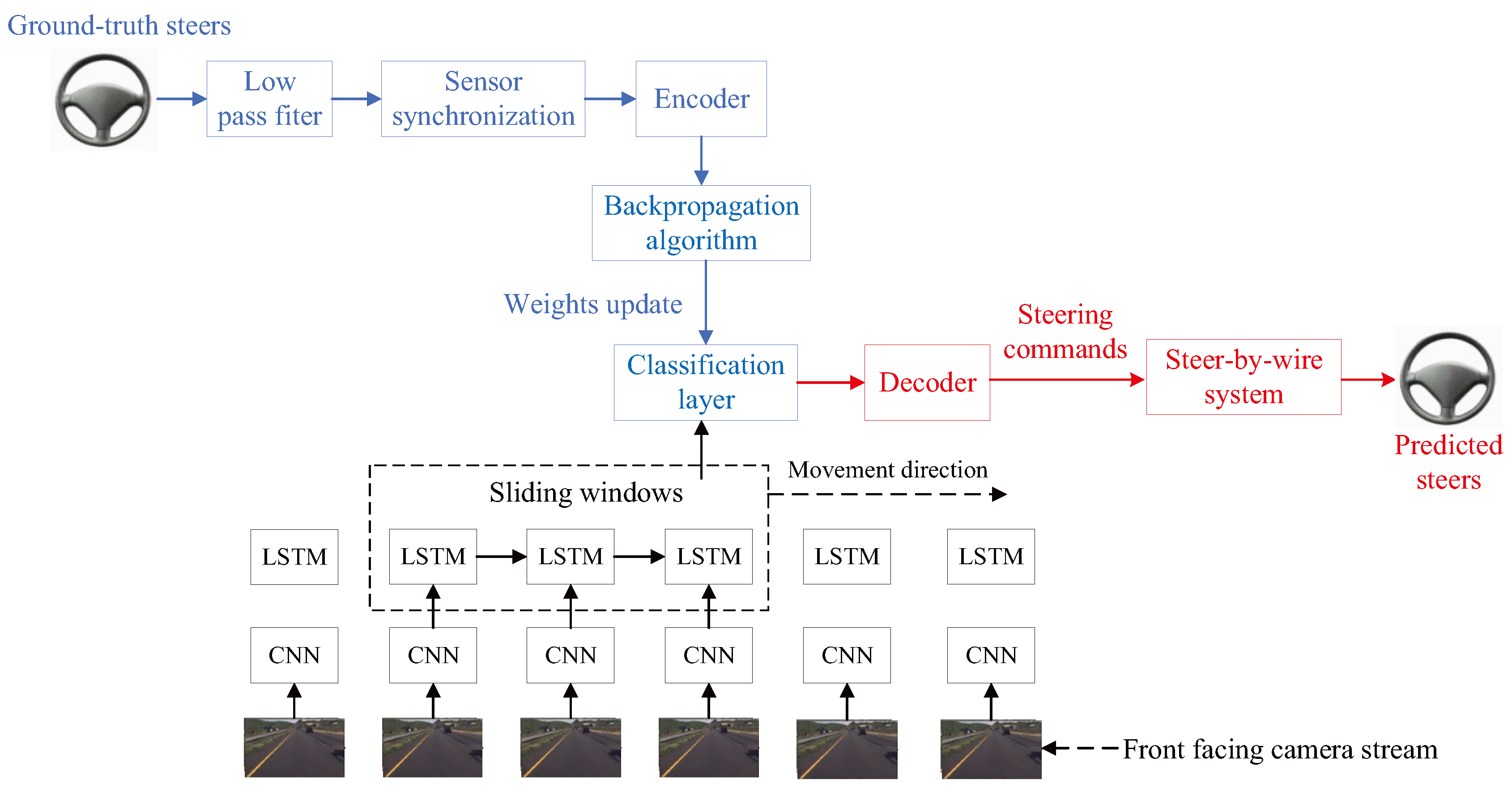
Motion control of a vehicle is one of the most fundamental tasks in self-driving cars. Deep learning-based methods are often used as the solutions in the end-to-end control system for self-driving cars, which directly maps sensory data to steering commands. For example, Eraqi, et al. [80] proposed a composite neural network, which is used to estimate the angle of the steering wheel. This network includes a CNN and an LSTM network, which uses the camera as input. The CNN is used to process the camera images frame by frame. The features of the driving scene are extracted by the CNN and then passed into a stack of LSTM layers. The temporal dependence of these features can be learned by the LSTM network. At last, the steering angle prediction is carried out by the output layer. An overview of the block diagram of the system proposed in [80] is shown in Figure 19.

During the training process of the method in [80], the ground-truth steering angle $\varphi$ is encoded as following sine wave function:

$$Y_i=sin\left(\frac{2\pi \left(i-1\right)}{N-1}-\frac{\varphi \pi }{2{\varphi }_{max}}\right),1\le i\le N,$$

(19)

where $Y_i$ is the activation of the i-th output neuron and N is the number of output neurons. In this method, a least squares regression is used in the classification layer, to fit the predicted function. In the process of deployment, the steering angle is output based on the results of the least squares regression.

4.4.3. Pedestrian Detection

Pedestrian detection is very important for self-driving cars, which can be used to obtain the location of individuals on the road. There are many advantages of the deep learning-based pedestrian detection methods in discriminative and representative feature learning. So, the pedestrian detection methods based on deep learning have been studied extensively. For example, Shen et al. [81] proposed a single-shot pedestrian detection method using a multi-receptive field-based framework. The framework of the pedestrian detection in [81] is shown in Figure 20. First, the image is used as the input of the Visual Geometry Group (VGG) network. Then, the multi-resolution and multi-receptive field feature pyramid is built.

As shown in Figure 20, a multi-receptive pooling pyramid (MRPP) module is proposed to extract feature maps. There are four max-pooling layers in this MRPP module, which are used to deal with the spatial size of the final VGG feature maps. The MRPP module will output five feature maps with different spatial resolutions. Then, a Graph CNN (GCN) module is used to handle the occlusion problem based on the outputs of the MRPP module and one VGG feature. The final detection results can be obtained based on the single-shot multi-box detection (SSD) algorithm and the non-maximum suppression module.

In the training process of the method in [81], there are two parts in the objective function, namely the classification loss (denoted as $L_{cls}$) and the localisation loss (denoted as $L_{loc}$). $L_{cls}$ is a multiple classes Softmax loss, which is defined as follows:

$$L_{cls}=-\frac{1}{N}\sum _{i=1}^N\sum _{j=1}^k{t}_{i,j}log\left(p_{i,j}\right)=-\frac{1}{N}\sum _{i=1}^{N}ylog\left(p_{i,j}\right),$$

(20)

where $t_{i,j}$ denotes the indicator of the i-th sample in class j; $p_{i,j}$ is the predicted output; and y is the class label of the ground truth. $L_{loc}$ is a bounding box regression loss, which is defined as follows:

$$L_{loc}=\sum _{i=1}^N{t}_{i,j}{\mathrm{smooth}}_{L1}\left(p_{box},g_{box}\right),$$

(21)

where $p_{box}$ and $g_{box}$ are the parameters of the predicted and ground truth bounding box respectively. The total loss function is defined as follows:

$$L=L_{cls}+\lambda L_{loc},$$

(22)

where $\lambda$ is a balancing parameter of the two loss terms.

4.4.4. Traffic Signs and Lights Recognition

Traffic signs and lights recognition is an important task in the self-driving system. The traffic signs recognition can provide some helpful information for the navigation and safe driving (see Figure 21a). The traffic lights perception at intersections and crosswalks is a necessary function for self-driving cars to observe the traffic regulations and prevent fatal accidents (see Figure 21b). Deep learning methods have demonstrated prominent representation capacity, and achieved outstanding performance in the traffic sign and light recognition, which are reviewed simply as follows.

In the traffic signs recognition, Xu et al. [82] proposed a traffic signs recognition approach based on a CNN algorithm. First, the structural information of the traffic sign image is extracted based on the hierarchical significance detection method. Then, a neural network model is used to extract the features of the region of interest. Finally, the traffic sign is classified by the Softmax classifier to complete the detection of the traffic sign. Alghmgham et al. [83] designed a deep-learning-based architecture and applied it in the real-time traffic sign classification. The proposed architecture in [83] consists of two convolutional layers, two max-pooling layers, one dropout layer and three dense layers.

In the traffic lights recognition, Lee and Kim [84] proposed a DNN-based method to detect traffic lights in images. The detector in this paper has a DNN architecture of encoder-decoder. The encoder is used to generate feature maps from the images by the ResNet-101. Then, the decoder is used to generate a refined feature map from the results of the encoder, to output the final classification results for the traffic lights. Kim et al. [85] proposed a traffic light recognition method based on deep learning, which consists of a semantic segmentation network and a fully convolutional network. The semantic segmentation network is employed to detect traffic lights and the fully convolutional network is used for traffic light classification.

5. Future Directions

In recent years, deep learning has made a breakthrough in image recognition, and also promoted the increasing development of self-driving cars technology. It can be seen from the achievements of several scientific research organizations that the research on self-driving cars has made great progress. However, the applications of deep learning for self-driving cars still have many challenges, which need to be improved as follows:

(1) The samples problem of deep learning. The deep learning model is trained through samples. In order to achieve the required accuracy in the recognition task, a large number of correct samples are usually required to meet the needs of developers. The quantity and quality of data is still a problem for good generalization capability [86]. In addition, the development of more realistic virtual datasets is an open problem, which can be solved by recording real cases [87,88,89].

(2) The complexity problem of deep learning. The complexity of deep learning algorithms is described by the parameters of the model. The number of parameters in a deep learning model usually exceeds millions [90]. The deep learning model is considerably complex with various functions to realize, so it cannot be trained on simple equipment. Embedded hardware needs strong communication and computing capabilities. So the hardware of self-driving cars needs to be improved, and the tradeoff of the performance and the price should be considered.

(3) The robustness problem of deep learning. The applications of self-driving cars based on deep learning methods rely on the images obtained during driving. However, the pictures acquired in the process of moving are easy to be interfered with by occlusion and illumination, which decreases the recognition accuracy. Robustness against influences is a key challenge.

(4) The real-time problem of deep learning. The processing ability of the human brain is still beyond the range of current deep learning. The perception speed to surrounding environment information of the autonomous driving model is far less than the speed of human response, so the real-time requirement still needs to be further improved.

(5) The high-dimensional state-space problem of deep learning. Real-world problems usually involve high-dimensional continuous state space (a large number of state or actions) [91]. When faced with the overwhelming set of different states and/or actions, it will be difficult to solve optimization problems and seriously restrict the development of practical applications based on deep learning. An effective approach to deal with such problems remains a challenge.

(6) The 3D point cloud data processing based on deep learning. The methods focused on in this paper are all based on image sensors. The range sensor is also the main sensor used in self-driving cars. The 3D point clouds can be obtained based on range sensors (such as LiDAR), which are useful for scene understanding [92], object detection [93], and so on. Deep learning is good at processing the point cloud data too, however, it is faced with many problems like arraying irregularly in space. In the future, there are still many challenges, including how to further solve the disorder problem of the point cloud data, the sampling problem of non-uniform distribution and the noise problem of original data.

(7) The road support system based on deep learning. The road support system is a scheduling and auxiliary system, which is often installed at the city traffic control center. So the tasks of the road support system are different from those of self-driving cars introduced above, such as vehicle detection and identification, pedestrian detection, and license plate recognition [94]. The road support system can provide more accurate and effective assistance for self-driving cars. Because the road support system can obtain much more information than the self-driving car, it is a new challenge for the methods based on deep learning.

The ultimate goal for the development of self-driving cars is to build an automatic platform capable of real-time, all-day and efficient driving service. Driverless technology can greatly improve social productivity, generate huge social benefits, and improve the way people travel, to make a better living environment. So there are lots of problems that need to be solved efficiently, which include two sides, namely the applications of self-driving cars based on deep learning and the improvements of deep learning algorithms. Thus, self-driving cars based on deep learning are still on the road.

6. Conclusions

In this survey, the latest advances in the development of autonomous driving systems based on deep learning techniques were analyzed. This paper first introduced the development of deep learning and self-driving cars in recent years, as well as the mainstream architecture of self-driving cars. Then the most common network architectures in deep learning used for self-driving cars were described. Furthermore, the current research and applications of deep learning in the field of self-driving cars were elaborated and the details of some representative approaches in the applications of self-driving cars were given out. Finally, the key problems and challenges in deep learning for self-driving cars were analyzed. Because the number of the literature is large and is still growing in this area, many good methods based on deep learning have not been included to focus on some of the key issues in this field.

It is clear that deep learning methods will become one of the hottest research topics in the self-driving car field, including theory and application research. The deep learning will be able to further improve the intelligence and autonomy of self-driving cars, and can solve some bottle-necks of traditional technologies, such as the accuracy, robustness, and safety. Currently, many basic problems of self-driving cars based on deep learning have been explored and the results are exciting, which show the potential of deep learning. However, there are still lots of problems that should be further studied, such as real-time problems, reliability problems, and so on.

References

- Duarte, F. Self-driving cars: A city perspective. Sci. Robot. 2019, 4. [Google Scholar] [CrossRef]
- Shakhatreh, H.; Sawalmeh, A.H.; Al-Fuqaha, A.; Dou, Z.; Almaita, E.; Khalil, I.; Othman, N.S.; Khreishah, A.; Guizani, M. Unmanned aerial vehicles (UAVs): A survey on civil applications and key research challenges. IEEE Access 2019, 7, 48572–48634. [Google Scholar] [CrossRef]
- Clements, L.M.; Kockelman, K.M. Economic effects of automated vehicles. Trans. Res. Rec. 2017, 2606, 106–114. [Google Scholar] [CrossRef]
- Hussain, R.; Zeadally, S. Autonomous cars: research results, issues, and future challenges. IEEE Commun. Surv. Tutor. 2019, 21, 1275–1313. [Google Scholar] [CrossRef]
- Xue, J.R.; Fang, J.W.; Zhang, P. A survey of scene understanding by event reasoning in autonomous driving. Int. J. Autom. Comput. 2018, 15, 249–266. [Google Scholar] [CrossRef]
- Wang, Z.; Liu, K.; Li, J.; Zhu, Y.; Zhang, Y. Various frameworks and libraries of machine learning and deep learning: A survey. Arch. Comput. Methods Eng. 2019. [Google Scholar] [CrossRef]
- Guo, G.; Zhang, N. A survey on deep learning based face recognition. Comput. Vis. Image Underst. 2019, 189, 102805. [Google Scholar] [CrossRef]
- Greenblatt, N.A. Self-driving cars and the law. IEEE Spect. 2016, 53, 46–51. [Google Scholar] [CrossRef]
- Bengio, Y.I.; Goodfellow, J.; Courville, A. Deep Learning; MIT Press: Cambridge, MA, USA, 2016. [Google Scholar]
- Birdsall, M. Google and ITE: The road ahead for self-driving cars. ITE J. (Inst. Transp. Eng.) 2014, 84, 36–39. [Google Scholar]
- Dikmen, M.; Burns, C. Trust in autonomous vehicles: The case of Tesla autopilot and summon. In Proceedings of the 2017 IEEE International Conference on Systems, Man, and Cybernetics, SMC 2017, Banff, AB, Canada, 5–8 October 2017; pp. 1093–1098. [Google Scholar]
- Coelingh, E.; Nilsson, J.; Buffum, J. Driving tests for self-driving cars. IEEE Spectr. 2018, 55, 41–45. [Google Scholar] [CrossRef]
- Park, J.; Nam, C.; Kim, H.j. Exploring the key services and players in the smart car market. Telecommun. Policy 2019, 43, 101819. [Google Scholar] [CrossRef]
- Toschi, A.; Sanic, M.; Leng, J.; Chen, Q.; Wang, C.; Guo, M. Characterizing perception module performance and robustness in production-scale autonomous driving system. In Proceedings of the 16th IFIP WG 10.3 International Conference on Network and Parallel Computing, Hohhot, China, 23–24 August 2019; pp. 235–247. [Google Scholar]
- Li, Y.; Wang, J.; Xing, T.; Liu, T.; Li, C.; Su, K. TAD16K: An enhanced benchmark for autonomous driving. In Proceedings of the 24th IEEE International Conference on Image Processing, Beijing, China, 17–20 September 2017; pp. 2344–2348. [Google Scholar]
- Yue, L.; Abdel-Aty, M.; Wu, Y.; Wang, L. Assessment of the safety benefits of vehicles advanced driver assistance, connectivity and low level automation systems. Accident Anal. Prev. 2018, 117, 55–64. [Google Scholar] [CrossRef] [PubMed]
- Bylykbashi, K.; Qafzezi, E.; Ikeda, M.; Matsuo, K.; Barolli, L. Fuzzy-based driver monitoring system (FDMS): Implementation of two intelligent FDMSs and a testbed for safe driving in VANETs. Future Gener. Comput. Syst. 2020, 105, 665–674. [Google Scholar] [CrossRef]
- Schnelle, S.; Wang, J.; Jagacinski, R.; Su, H.j. A feedforward and feedback integrated lateral and longitudinal driver model for personalized advanced driver assistance systems. Mechatronics 2018, 50, 177–188. [Google Scholar] [CrossRef]
- Paden, B.; Cap, M.; Yong, S.Z.; Yershov, D.; Frazzoli, E. A survey of motion planning and control techniques for self-driving urban vehicles. IEEE Trans. Intell. Veh. 2016, 1, 33–55. [Google Scholar] [CrossRef] [Green Version]
- Mittal, S. A Survey on optimized implementation of deep learning models on the NVIDIA Jetson platform. J. Syst. Arch. 2019, 97, 428–442. [Google Scholar] [CrossRef]
- Jones, L. Driverless when and cars: Where? Eng. Technol. 2017, 12, 36–40. [Google Scholar] [CrossRef]
- Dekhtiar, J.; Durupt, A.; Bricogne, M.; Eynard, B.; Rowson, H.; Kiritsis, D. Deep learning for big data applications in CAD and PLM research review, opportunities and case study. Comput. Ind. 2018, 100, 227–243. [Google Scholar] [CrossRef]
- Ni, J.; Wang, K.; Cao, Q.; Khan, Z.; Fan, X. A memetic algorithm with variable length chromosome for robot path planning under dynamic environments. Int. J. Robot. Autom. 2017, 32, 414–424. [Google Scholar] [CrossRef] [Green Version]
- Ni, J.; Wu, L.; Fan, X.; Yang, S.X. Bioinspired intelligent algorithm and its applications for mobile robot control: A survey. Comput. Intell. Neurosci. 2016, 2016, 3810903. [Google Scholar] [CrossRef] [Green Version]
- McCall, R.; McGee, F.; Mirnig, A.; Meschtscherjakov, A.; Louveton, N.; Engel, T.; Tscheligi, M. A taxonomy of autonomous vehicle handover situations. Transp. Res. Part A Policy Pract. 2019, 124, 507–522. [Google Scholar] [CrossRef]
- Liu, M.; Grana, D. Accelerating geostatistical seismic inversion using TensorFlow: A heterogeneous distributed deep learning framework. Comput. Geosci. 2019, 124, 37–45. [Google Scholar] [CrossRef]
- Zhao, B.; Feng, J.; Wu, X.; Yan, S. A survey on deep learning-based fine-grained object classification and semantic segmentation. Int. J. Autom. Comput. 2017, 14, 119–135. [Google Scholar] [CrossRef]
- Zhong, Z.; Li, J.; Luo, Z.; Chapman, M. Spectral-spatial residual network for hyperspectral image classification: A 3-D deep learning framework. IEEE Trans. Geosci. Remote Sens. 2018, 56, 847–858. [Google Scholar] [CrossRef]
- Agrawal, P.; Ganapathy, S. Modulation filter learning using deep variational networks for robust speech recognition. IEEE J. Sel. Top. Sign. Process. 2019, 13, 244–253. [Google Scholar] [CrossRef]
- Zhang, Z.; Geiger, J.; Pohjalainen, J.; Mousa, A.E.D.; Jin, W.; Schuller, B. Deep learning for environmentally robust speech recognition: An overview of recent developments. ACM Trans. Intell. Syst. Technol. 2018, 9, 49. [Google Scholar] [CrossRef]
- Young, T.; Hazarika, D.; Poria, S.; Cambria, E. Recent trends in deep learning based natural language processing. IEEE Comput. Intell. Mag. 2018, 13, 55–75. [Google Scholar] [CrossRef]
- Sun, S.; Luo, C.; Chen, J. A review of natural language processing techniques for opinion mining systems. Inform. Fus. 2017, 36, 10–25. [Google Scholar] [CrossRef]
- Yu, Y.; Si, X.; Hu, C.; Zhang, J. A review of recurrent neural networks: LSTM cells and network architectures. Neural Comput. 2019, 31, 1235–1270. [Google Scholar] [CrossRef]
- Gers, F.A.; Schmidhuber, J.; Cummins, F. Learning to forget: Continual prediction with LSTM. In Proceedings of the 1999 the 9th International Conference on ‘Artificial Neural Networks (ICANN99)’, Edinburgh, UK, 7–10 September 1999; Volume 2, pp. 850–855. [Google Scholar]
- Bouwmans, T.; Javed, S.; Sultana, M.; Jung, S.K. Deep neural network concepts for background subtraction: A systematic review and comparative evaluation. Neural Netw. 2019, 117, 8–66. [Google Scholar] [CrossRef] [Green Version]
- Fu, J.; Liu, J.; Li, Y.; Bao, Y.; Yan, W.; Fang, Z.; Lu, H. Contextual deconvolution network for semantic segmentation. Pattern Recognit. 2020, 101, 107152. [Google Scholar] [CrossRef]
- Woo, J.; Kim, N. Collision avoidance for an unmanned surface vehicle using deep reinforcement learning. Ocean Eng. 2020, in press. [Google Scholar] [CrossRef]
- Ding, Y.; Ma, L.; Ma, J.; Suo, M.; Tao, L.; Cheng, Y.; Lu, C. Intelligent fault diagnosis for rotating machinery using deep Q-network based health state classification: A deep reinforcement learning approach. Adv. Eng. Inform. 2019, 42, 100977. [Google Scholar] [CrossRef]
- Ni, J.; Liu, M.; Ren, L.; Yang, S.X. A multiagent Q-learning-based optimal allocation approach for urban water resource management system. IEEE Trans. Autom. Sci. Eng. 2014, 11, 204–214. [Google Scholar] [CrossRef]
- Ni, J.; Li, X.; Hua, M.; Yang, S.X. Bioinspired neural network-based Q-learning approach for robot path planning in unknown environments. Int. J. Robot. Autom. 2016, 31, 464–474. [Google Scholar] [CrossRef]
- Wen, S.; Zhao, Y.; Yuan, X.; Wang, Z.; Zhang, D.; Manfredi, L. Path planning for active SLAM based on deep reinforcement learning under unknown environments. Intell. Serv. Robot. 2020, in press. [Google Scholar] [CrossRef]
- Mnih, V.; Kavukcuoglu, K.; Silver, D.; Rusu, A.A.; Veness, J.; Bellemare, M.G.; Graves, A.; Riedmiller, M.; Fidjeland, A.K.; Ostrovski, G.; et al. Human-level control through deep reinforcement learning. Nature 2015, 518, 529–533. [Google Scholar] [CrossRef]
- Liu, H.; Sun, F.; Zhang, X. Robotic material perception using active multimodal fusion. IEEE Trans. Indust. Electron. 2019, 66, 9878–9886. [Google Scholar] [CrossRef]
- Zhang, X.; Zhou, M.; Qiu, P.; Huang, Y.; Li, J. Radar and vision fusion for the real-time obstacle detection and identification. Indust. Robot 2019, 46, 391–395. [Google Scholar] [CrossRef]
- Kriechbaumer, T.; Blackburn, K.; Breckon, T.P.; Hamilton, O.; Casado, M.R. Quantitative evaluation of stereo visual odometry for autonomous vessel localisation in inland waterway sensing applications. Sensors 2015, 15, 31869–31887. [Google Scholar] [CrossRef] [Green Version]
- Mancini, M.; Costante, G.; Valigi, P.; Ciarfuglia, T.A. J-MOD2: Joint monocular obstacle detection and depth estimation. IEEE Robot. Autom. Lett. 2018, 3, 1490–1497. [Google Scholar]
- Chen, H. Monocular vision-based obstacle detection and avoidance for a multicopter. IEEE Access 2019, 7, 167869–167883. [Google Scholar]
- Parmar, Y.; Natarajan, S.; Sobha, G. DeepRange: Deep-learning-based object detection and ranging in autonomous driving. IET Intell. Trans. Syst. 2019, 13, 1256–1264. [Google Scholar]
- Scharstein, D.; Szeliski, R. A taxonomy and evaluation of dense two-frame stereo correspondence algorithms. Int. J. Comput. Vis. 2002, 47, 7–42. [Google Scholar]
- Žbontar, J.; Lecun, Y. Stereo matching by training a convolutional neural network to compare image patches. J. Mach. Learn. Res. 2016, 17, 1–32. [Google Scholar]
- Nguyen, T.P.; Jeon, J.W. Wide context learning network for stereo matching. Signal Process. Image Commun. 2019, 78, 263–273. [Google Scholar]
- Zhang, G.; Zhu, D.; Shi, W.; Ye, X.; Li, J.; Zhang, X. Multi-dimensional residual dense attention network for stereo matching. IEEE Access 2019, 7, 51681–51690. [Google Scholar]
- Kendall, A.; Martirosyan, H.; Dasgupta, S.; Henry, P.; Kennedy, R.; Bachrach, A.; Bry, A. End-to-end learning of geometry and context for deep stereo regression. In Proceedings of the 16th IEEE International Conference on Computer Vision, ICCV 2017, Venice, Italy, 22–29 October 2017. [Google Scholar]
- Dairi, A.; Harrou, F.; Sun, Y.; Senouci, M. Obstacle detection for intelligent transportation systems using deep stacked autoencoder and k-nearest neighbor scheme. IEEE Sens. J. 2018, 18, 5122–5132. [Google Scholar]
- Mancini, M.; Costante, G.; Valigi, P.; Ciarfuglia, T.A. Fast robust monocular depth estimation for obstacle detection with fully convolutional networks. In Proceedings of the 2016 IEEE/RSJ International Conference on Intelligent Robots and Systems, IROS 2016, Daejeon, Korea, 9–14 October 2016; Volume 2016-November, pp. 4296–4303. [Google Scholar]
- Jia, B.; Feng, W.; Zhu, M. Obstacle detection in single images with deep neural networks. Signal Image Video Process. 2016, 10, 1033–1040. [Google Scholar]
- Zhong, Y.; Li, H.; Dai, Y. Open-world stereo video matching with deep RNN. In Proceedings of the 15th European Conference on Computer Vision, ECCV 2018, Munich, Germany, 8–14 September 2018. [Google Scholar]
- Jie, Z.; Wang, P.; Ling, Y.; Zhao, B.; Wei, Y.; Feng, J.; Liu, W. Left-right comparative recurrent model for stereo matching. In Proceedings of the 31st Meeting of the IEEE/CVF Conference on Computer Vision and Pattern Recognition, Salt Lake City, UT, USA, 18–22 June 2018. [Google Scholar]
- Chen, L.; Zhan, W.; Tian, W.; He, Y.; Zou, Q. Deep integration: A multi-label architecture for road scene recognition. IEEE Trans. Image Process. 2019, 28, 4883–4898. [Google Scholar]
- Wang, L.; Guo, S.; Huang, W.; Xiong, Y.; Qiao, Y. Knowledge guided disambiguation for large-scale scene classification with multi-resolution CNNs. IEEE Trans. Image Process. 2017, 26, 2055–2068. [Google Scholar] [CrossRef] [Green Version]
- Tang, P.; Wang, H.; Kwong, S. G-MS2F: GoogLeNet based multi-stage feature fusion of deep CNN for scene recognition. Neurocomputing 2017, 225, 188–197. [Google Scholar] [CrossRef]
- Byeon, W.; Breuel, T.M.; Raue, F.; Liwicki, M. Scene labeling with LSTM recurrent neural networks. In Proceedings of the IEEE Conference on Computer Vision and Pattern Recognition, CVPR 2015, Boston, MA, USA, 7–12 June 2015. [Google Scholar]
- Zhang, L.; Li, L.; Pan, X.; Cao, Z.; Chen, Q.; Yang, H. Multi-level ensemble network for scene recognition. Multimed. Tools Appl. 2019, 78, 28209–28230. [Google Scholar] [CrossRef]
- Liu, S.; Tian, G.; Xu, Y. A novel scene classification model combining ResNet based transfer learning and data augmentation with a filter. Neurocomputing 2019, 338, 191–206. [Google Scholar] [CrossRef]
- Cheng, X.; Lu, J.; Feng, J.; Yuan, B.; Zhou, J. Scene recognition with objectness. Pattern Recognit. 2018, 74, 474–487. [Google Scholar] [CrossRef]
- Sun, N.; Li, W.; Liu, J.; Han, G.; Wu, C. Fusing object semantics and deep appearance features for scene recognition. IEEE Trans. Circuits Syst. Video Technol. 2019, 29, 1715–1728. [Google Scholar] [CrossRef]
- John, V.; Liu, Z.; Mita, S.; Guo, C.; Kidono, K. Real-time road surface and semantic lane estimation using deep features. Signal Image Video Process. 2018, 12, 1133–1140. [Google Scholar] [CrossRef]
- Xiao, D.; Yang, X.; Li, J.; Islam, M. Attention deep neural network for lane marking detection. Knowl. Based Syst. 2020, 105584. [Google Scholar] [CrossRef]
- Kim, J.; Kim, J.; Jang, G.J.; Lee, M. Fast learning method for convolutional neural networks using extreme learning machine and its application to lane detection. Neural Netw. 2017, 87, 109–121. [Google Scholar] [CrossRef]
- Liu, J. Learning full-reference quality-guided discriminative gradient cues for lane detection based on neural networks. J. Vis. Commun. Image Represent. 2019, 65, 102675. [Google Scholar] [CrossRef]
- Li, J.; Mei, X.; Prokhorov, D.; Tao, D. Deep neural network for structural prediction and lane detection in traffic scene. IEEE Trans. Neural Networks Learn. Syst. 2017, 28, 690–703. [Google Scholar] [CrossRef] [PubMed] [Green Version]
- Tian, Y.; Gelernter, J.; Wang, X.; Chen, W.; Gao, J.; Zhang, Y.; Li, X. Lane marking detection via deep convolutional neural network. Neurocomputing 2018, 280, 46–55. [Google Scholar] [CrossRef] [PubMed]
- Neven, D.; De Brabandere, B.; Georgoulis, S.; Proesmans, M.; Van Gool, L. Towards end-to-end lane detection: An instance segmentation approach. In Proceedings of the 2018 IEEE Intelligent Vehicles Symposium, IV 2018, Changshu, China, 26–30 June 2018. [Google Scholar]
- Yang, W.; Cheng, Y.; Chung, P. Improved lane detection with multilevel features in branch convolutional neural networks. IEEE Access 2019, 7, 173148–173156. [Google Scholar] [CrossRef]
- Zou, Q.; Jiang, H.; Dai, Q.; Yue, Y.; Chen, L.; Wang, Q. Robust lane detection from continuous driving scenes using deep neural networks. IEEE Trans. Veh. Technol. 2020, 69, 41–54. [Google Scholar] [CrossRef] [Green Version]
- Ghafoorian, M.; Nugteren, C.; Baka, N.; Booij, O.; Hofmann, M. EL-GAN: Embedding loss driven generative adversarial networks for lane detection. In Proceedings of the 15th European Conference on Computer Vision, ECCV 2018, Munich, Germany, 8–14 September 2018; pp. 256–272. [Google Scholar]
- Ni, J.; Wu, L.; Shi, P.; Yang, S.X. A dynamic bioinspired neural network based real-time path planning method for autonomous underwater vehicles. Comput. Intell. Neurosci. 2017, 2017, 9269742. [Google Scholar] [CrossRef]
- Ni, J.; Yang, L.; Wu, L.; Fan, X. An improved spinal neural system-based approach for heterogeneous AUVs cooperative hunting. Int. J. Fuzzy Syst. 2018, 20, 672–686. [Google Scholar] [CrossRef]
- Yu, L.; Shao, X.; Wei, Y.; Zhou, K. Intelligent land-vehicle model transfer trajectory planning method based on deep reinforcement learning. Sensors (Switzerland) 2018, 18, 2905. [Google Scholar]
- Eraqi, H.M.; Moustafa, M.N.; Honer, J. End-to-end deep learning for steering autonomous vehicles considering temporal dependencies. In Proceedings of the 31st Conference on Neural Information Processing Systems (NIPS 2017), MLITS Workshop, Long Beach, CA, USA, 4–9 December 2017. [Google Scholar]
- Shen, C.; Zhao, X.; Fan, X.; Lian, X.; Zhang, F.; Kreidieh, A.R.; Liu, Z. Multi-receptive field graph convolutional neural networks for pedestrian detection. IET Intell. Trans. Syst. 2019, 13, 1319–1328. [Google Scholar] [CrossRef]
- Xu, H.; Srivastava, G. Automatic recognition algorithm of traffic signs based on convolution neural network. Multimed. Tools Appl. 2020, in press. [Google Scholar] [CrossRef]
- Alghmgham, D.A.; Latif, G.; Alghazo, J.; Alzubaidi, L. Autonomous traffic sign (ATSR) detection and recognition using deep CNN. Procedia Comput. Sci. 2019, 163, 266–274. [Google Scholar] [CrossRef]
- Lee, E.; Kim, D. Accurate traffic light detection using deep neural network with focal regression loss. Image Vis. Comput. 2019, 87, 24–36. [Google Scholar] [CrossRef]
- Kim, H.K.; Yoo, K.Y.; Park, J.H.; Jung, H.Y. Traffic light recognition based on binary semantic segmentation network. Sensors 2019, 19, 1700. [Google Scholar] [CrossRef] [Green Version]
- Testolin, A.; Stoianov, I.; Zorzi, M. Letter perception emerges from unsupervised deep learning and recycling of natural image features. Nat. Hum. Behav. 2017, 1, 657–664. [Google Scholar] [CrossRef]
- Fraga-Lamas, P.; Ramos, L.; Mondejar-Guerra, V.; Fernandez-Carames, T.M. A review on IoT deep learning UAV systems for autonomous obstacle detection and collision avoidance. Remote Sens. 2019, 11, 2144. [Google Scholar] [CrossRef] [Green Version]
- Micucci, A.; Mantecchini, L.; Sangermano, M. Analysis of the relationship between turning signal detection and motorcycle driver’s characteristics on urban roads; A case study. Sensors 2019, 19, 1802. [Google Scholar] [CrossRef] [Green Version]
- Micucci, A.; Sangermano, M. A study on cyclists behaviour and bicycles kinematic. Int. J. Trans. Dev. Integr. 2020, 4, 14–28. [Google Scholar] [CrossRef]
- Khamparia, A.; Singh, K.M. A systematic review on deep learning architectures and applications. Expert Syst. 2019, 36, e12400. [Google Scholar] [CrossRef]
- Carrio, A.; Sampedro, C.; Rodriguez-Ramos, A.; Campoy, P. A review of deep learning methods and applications for unmanned aerial vehicles. J. Sens. 2017, 2017, 3296874. [Google Scholar] [CrossRef]
- Zhang, R.; Li, G.; Li, M.; Wang, L. Fusion of images and point clouds for the semantic segmentation of large-scale 3D scenes based on deep learning. ISPRS J. Photogram. Remote Sens. 2018, 143, 85–96. [Google Scholar] [CrossRef]
- Yang, Y.; Chen, F.; Wu, F.; Zeng, D.; Ji, Y.M.; Jing, X.Y. Multi-view semantic learning network for point cloud based 3D object detection. Neurocomputing 2020, in press. [Google Scholar] [CrossRef]
- Sirohi, D.; Kumar, N.; Rana, P.S. Convolutional neural networks for 5G-enabled intelligent transportation system: A systematic review. Comput. Commun. 2020, 153, 459–498. [Google Scholar] [CrossRef]
Figure 1.
Self-driving cars of Google and Tesla: (a) Google’s self-driving car; (b) Tesla’s self-driving car.
Figure 2.
Self-driving cars of the companies in China: (a) Baidu’s self-driving car; (b) Tencent’s self-driving car.
Figure 3.
The overall technical framework of self-driving cars with a Level3 or higher autonomy system.
Figure 4.
The NVIDIA DRIVE PX2 driverless car platform.
Figure 5.
The network structure of Convolutional Neural Network.
Figure 6.
The network structure of Recurrent Neural Network (RNN).
Figure 7.
The structure of the traditional Auto-Encoder network (AE).
Figure 8.
The structure of the reinforcement learning (RL).
Figure 9.
The classification of the deep learning methods used in the field of self-driving cars.
Figure 10.
Binocular visual obstacle detection flow chart.
Figure 11.
The structure of MC-CNN proposed in [50].
Figure 12.
Examples of the disparity results by MC-CNN in [50]: (a) error of 3.73%; (b) error of 2.36%.
Figure 13.
The impacts of weather: (a) bad weather; (b) good weather.
Figure 14.
The examples of various scenes: (a) urban main road; (b) suburban road; (c) mountain road; (d) city street.
Figure 15.
The structure of multi-resolution CNN proposed in [60].
Figure 16.
The training and testing process of the method in [67].
Figure 17.
The results of lane prediction based on the method presented in [67].
Figure 18.
The flow chart of the method proposed in [79].
Figure 19.
A overview of the block diagram of the system proposed in [80].
Figure 20.
The framework of the pedestrian detection in [81].
Figure 21.
The examples of various traffic signs and lights: (a) traffic signs; (b) traffic lights.