
Simulation-Based Business Valuation: Methodical Implementation in the Valuation Practice

International School of Finance (IFS), Nuertingen-Geislingen University, Sigmaringer Straße 25, 72622 Nürtingen, Germany
J. Risk Financial Manag. 2022, 15(5), 200; https://doi.org/10.3390/jrfm15050200
Submission received: 23 March 2022
/
Revised: 8 April 2022
/
Accepted: 20 April 2022
/
Published: 26 April 2022
(This article belongs to the Special Issue Empirical Corporate Finance: Opportunities and Challenges)
Abstract
:The simulation-based company valuation values a company on the basis of the risks actually present in the company without having to derive them from the capital market data. The simulation-based company valuation takes into account the market imperfections, such as the probability of insolvency or the lack of diversification, and fulfils the legal requirements and auditing standards for a company valuation. The simulation-based company valuation is an alternative to the CAPM-based company valuation, which, under the assumption of perfect capital markets, derives the risks through capital market comparisons. A simulation-based business valuation has many advantages and is particularly suitable for valuing medium-sized companies, start-ups, companies in a crisis, and for integrating country-specific risks into business valuations. Due to the internationally widespread use of the CAPM, a simulation-based company valuation is still rarely used in practice. This article shows which valuation formulas are necessary for the application of a simulation-based company valuation. These are used for both the certainty equivalent method and for the risk premium method. In a concrete and valuation example, the simulation-based business planning and company valuation is carried out, and the derived valuation formulas are applied in a way that allows a transfer to concrete valuation cases in practice. It is shown that the certainty equivalent method and the risk premium method lead to identical company values.
1. Introduction
Simulation-based business valuations have been in discussion for some time as an alternative to the CAPM-based business valuation (see Gleißner and Ernst 2019 for an English summary of the research and the literature cited there). The simulation-based business valuation has the advantage of capturing the company-specific risk position by means of an unbiased planning (Gleißner 2021). This makes it possible to derive a company value that reflects the actual risk situation in the company (Gleißner 2020). The simulation-based company valuation is especially suitable for the valuation of medium-sized companies, start-up companies, companies in a crisis, and for the integration of country-specific risks in the company valuation. A CAPM-based company valuation, on the other hand, calculates the risk in a company via the capital market route under the assumption of perfect capital markets, and is particularly suitable for the valuation of listed companies. Despite the methodological superiority of the simulation-based company valuation, it is, still, rarely used in practice and applied to valuation examples.
The value of a company corresponds to the market price only in perfect and complete capital markets (Shiller 1981; Brennan and Wang 2010); therefore, business valuation techniques are necessary to assign a value to the future cash flows graded as higher risk. The Discounted Cash Flow (DCF) method is the most common and important method for this purpose. The DCF method does not require a utility function. It is based on the ideal market calculations in a complete (e.g., arbitrage-free) and perfect capital market. This allows a perfect duplication of the cash flow streams to be valued; however, this approach requires that an infinite number of possible future conditions are modelled in order to obtain a perfect replication of cash flows.
The reason for the high importance of the CAPM in capital market-oriented valuation theory is that it does not assume completeness of the capital market. Furthermore, the CAPM provides with the Beta factor a simple risk parameter which is based on the (μ, σ)-principle (Dorfleitner and Gleißner 2018, pp. 4–5). The risk is derived from the historical fluctuations in stock returns incorporated in the beta factor. Empirical research shows, however, that neither the realized nor the expected stock returns can be explained by the beta factor alone (see the critique by Dempsey 2013). Although there are approaches to explain market imperfections such as bankruptcy costs, transaction costs, asymmetrically distributed information, boundedly rational behavior, and non-diversified portfolios (Shleifer 2000; Haugen 2002), a closed theory of the imperfect capital market does not yet exist. Alternatives to the CAPM, such as the well-known three-factor model of Fama and French (Fama and French 1993) and the five-factor model (Fama and French 2015), are only of limited use for the company valuation, as they lack a clear theoretical foundation (for empirical results, see Fama and French 2008; Fama and French 2012). It is important for the future development of the valuation theory that the mentioned “new” multi-factor models are no longer limited to evaluating only the capital market data. These models also take into account the characteristics of the companies to be valued (Zhang 2009; Novy-Marx 2013), such as profitability (return on equity), growth, or the probability of insolvency (distress factor), when deriving expected returns and the risk-adjusted discount rates; however, the specific relevant company characteristics remain to be critically analyzed, such as the risks associated with the company’s cash flows, which have so far still received little attention in the field of capital market research.
Due to the increasing imperfections in capital markets and the growing influence of risk management in companies, some valuation approaches have burgeoned in the recent years that, on the one hand, derive the risk scope of companies through risk analysis, and on the other hand, take into account the imperfections of real markets. These approaches include investment-theoretical valuation theory (Smith 1998; Hazen 2009 for extensive references) and simulation-based valuation theory (Gleißner and Ernst 2019 and the literature cited there). The investment-theoretical valuation theory assumes that the preferences of a decision-maker can be described as a neoclassical decision function. In practical applications, however, it is problematic that the valuation with the so-called “total models” presupposes a simultaneous optimization of all the options for action, and thus requires unrealistic demands on the level of information (for example Fishburn 1977; Tversky and Kahneman 1979). The simplifying “partial models” make it possible to reduce complexity, but they do not provide a method for deriving the risk-adequate discount rates (and in particular, no link to risk simulation and risk aggregation).
Based on the fundamental ideas of investment-theoretical valuation theory, “semi-investment-theoretical” valuation methods have been developed in recent years, which are also referred to as simulation-based methods. In practice, these methods are used to evaluate investments, companies, determine the rating, risk-bearing capacity, and risk coverage. The simulation-based methods also do not require the assumption of a perfect capital market, but they are much more practical than investment theory valuation methods. Simulation-based methods make it possible to use the DCF methods, commonly used in the valuation practice. Instead of information on the (historical) stock return fluctuations, such as the beta factor of the CAPM, the company-specific information from the risk analysis and risk aggregation is used to calculate unbiased planned values of cash flows and the risk-adequate cost of capital. The insolvency scenarios, possibly as a result of the risks, and thus the insolvency risk, can also be easily reflected in the valuation calculation.
Dorfleitner and Gleißner (2018), and Dorfleitner (2020), have presented the formal framework of the simulation-based valuation. It has not yet been shown how the connection to the DCF models used in the valuation practice can be established. Gleißner and Ernst (2019) describe important basics of the simulation-based valuation and demonstrate them with a simple example, which, however, does not answer questions of implementation in a concrete valuation example. Furthermore, they do not discuss which formulas are used in the certainty equivalent method and the risk premium method to arrive at identical company values. In this paper, the necessary formulas are derived. They show how risk information from the simulation as well as the simulated insolvency probability and the growth rate are taken into account in the terminal value formula. Furthermore, through a retrograde valuation in the certainty equivalent method, the certainty equivalent of each period will be included in the formula in order to be able to discount with the risk-free interest rate. In order to increase the acceptance of the simulation-based business valuation in practice, the application of the formulas presented here is demonstrated in a practical valuation case.
The paper is structured as follows. First, the simulation-based business valuation is briefly introduced, and it is shown how the valuation can be carried out using the certainty equivalent method and the risk premium method. The relationship between the two methods is explained by deriving the cost of capital for the risk premium method from the certainty equivalent method. Subsequently, the valuation equations for the certainty equivalent method and the risk premium method are calculated with the help of a retrograde valuation; thereafter, the valuation formula for the terminal value and the valuation formula for the detailed planning period are presented for both methods. In a practical example, we demonstrate how a professional simulation-based business valuation can be carried out. Finally, the results are summarized, the limitations of the approach are discussed, and further fields of research are identified.
2. The Concept of the Simulation-Based Company Valuation
A simulation-based business valuation relies on information about the risks of the company itself, which are determined by means of risk analysis. Here, a distinction is made, not between systematic and unsystematic risks as is customary in the CAPM, but between the risks hedged and non-hedged in the company (Ernst and Häcker 2021). These risks are modelled within the business plan using suitable distribution functions, and they form the basis of unbiased business planning. After carrying out a Monte Carlo simulation, the risk measures are selected for the aggregated risks within the framework of a risk analysis. These risk measures provide the basis for risk processing in a simulation-based business valuation.
From this approach, the core features of a simulation-based business valuation can be derived:
- consideration of the corporate risks,
- and application of a Monte Carlo simulation for risk aggregation.
A simulation-based valuation does not initially imply a commitment to a specific valuation theoretical framework. If one chooses, as is in common practice, a semi-investment-theoretical valuation by means of an “imperfect replication” (Gleißner 2019; Dorfleitner and Gleißner 2018), all market constellations are from a high degree of market imperfection to a perfect and complete capital market (also the CAPM as a special case) can be modelled (Gleißner and Ernst 2019).
The frequency distributions resulting from the Monte Carlo simulation are each condensed to the expected value in the simulation-based valuation and the risk of the cash flows is expressed by a risk measure, such as standard deviation or value-at-risk. A risk-value model and the imperfect replication method can be used to calculate the risk-adequate present value of the cash flows, taking into account their (a) amount, (b) risk, and (c) timing.
The essential features and advantages of a simulation-based business valuation based on the analysis of the business risks can be summarized as follows (Gleißner 2021):
- Only simulation-based planning can derive the comprehensible, unbiased, expected values of cash flows.
- A plausibility check of the planning and planning logic is carried out through risk identification, risk quantification, and risk aggregation.
- With a simulation-based valuation, the effects of insolvency risk on the company value can be easily incorporated into the valuation model.
- A simulation-based business valuation enables the derivation of a risk-adequate cost of capital directly from the risk analysis of the simulation results.
- The simulation-based valuation is also a suitable basis for the preparation of entrepreneurial decisions.
- A simulation-based valuation is the only valuation method that meets the legal requirements and auditing standards for risk management.
The simulation-based company valuation can now be carried out with
- the certainty equivalent method or
- the risk premium method.
We start with the certainty equivalent method, since without this, the cost of capital for the risk premium method cannot be derived.
3. Valuation with the Certainty Equivalent Method
In the certainty equivalent method, a risk discount is deducted from the expected value of the cash flow. In this process, the expected future (uncertain) cash flows are transformed into certain cash flows. The resulting certainty equivalents are then discounted at the risk-free interest rate to obtain the present value of the cash flows or the enterprise value.
The certainty equivalent is the certain payment that provides the same utility as the uncertain cash flow (). A risk discount of the valuation-relevant cash flow is deducted from the expected value of the uncertain cash flows .
The risk discount itself is calculated as follows:
and is composed of the risk measure , the market price per unit of risk , and the degree of diversification .
is the risk associated with the cash flow, which is determined via the frequency distribution of the cash flow. The frequency distribution of the cash flow is determined with the help of a Monte Carlo simulation, which aggregates the non-hedged risks existing in a company via an integrated income statement and balance sheet planning. This makes it possible to carry out the following risk analysis from the company’s risk structure without having to rely on capital market data.
is the risk measure and it reflects the (aggregated) total risk of the cash flows, valued in monetary units. This can be the standard deviation of the cash flows or a value-at-risk measure. The risk measure of the cash flows is converted into a price of aggregate risk by multiplying it by the market price per unit risk . The price of the aggregated total risk is then multiplied by the share of the risks of the valuation object that the valuation subject has to bear.
The calculated certainty equivalents can now be used to calculate the enterprise value . In the certainty equivalent method, the certainty equivalents in the numerator are discounted with the risk-free interest rate in the denominator. The risk-free interest rate is used because the aggregated total risk has already been captured with the risk discount in the certainty equivalent.
Let us consider the certainty equivalent method in a single-period case.
As we can see, the certainty equivalent method clearly distinguishes between the risk preference (in the numerator) and the time preference (risk-free interest rate in the denominator). This is not the case with the risk premium method commonly used in practice, which we will address below.
4. Valuation with the Risk Premium Method
In the risk premium method, which is widely used in practice, the cash flows in the numerator are discounted with the risk-adjusted interest rate in the denominator. The risk premium is added to the risk-free interest rate to obtain cost of capital for discounting the future expected cash flows ().
is the normalised, aggregated total risk (in % of value = ), i.e., a measure of the return risk (like the standard deviation of the stock return). This is multiplied by the market price of the risk and the diversification factor of the valuation subject, as already explained above.
5. A Comparison between the Certainty Equivalent Method and the Risk Premium Method
The certainty equivalent method and the risk premium method are two approaches that incorporate the risk measure at different points in the valuation equation, but they result in identical company values. The application of the certainty equivalent method and the risk premium method have strengths and weaknesses for the practice of business valuation, which will be pointed out here.
First of all, it is very important to mention that the risk premium method is the commonly used method in business valuation practices. This is because the discounted cash flow (DCF) method originates from investment appraisal, in which one determines the net present value of an investment by discounting the future cash flows with a risk-adjusted interest rate; therefore, the risk premium method is applied here. This was then incorporated into the company valuation theory. Another important reason for using the risk premium method is that it is a standard method within the Capital Asset Pricing Model (CAPM) (for the use of a less common certainty equivalent variant of the CAPM, see Robichek and Myers 1966; Rubinstein 1973). As the CAPM has been the preferred model worldwide for calculating the premium risk, the risk premium method is also considered to be widely acceptable. Furthermore, the cost of capital is often used in the context of value-based management to control companies; therefore, there is a connection here in terms of the content. From an investor’s point of view, the cost of capital reflects the expected return on capital, so that here, too, a use of the risk premium method is popular.
A weakness of the risk premium method is the lack of separation between the risk and time preference. This can lead to valuation errors in certain valuation cases. These errors occur when the expected value of the cash flows is small or even negative compared with the risks (standard deviations). In such cases, the discounting of negative cash flows may occur. If the negative payments are discounted with a positive discount rate, the discounted value will erroneously be greater (less negative) than the expected value. In the certainty equivalent method, on the other hand, the certainty equivalent of a payment with a negative expected value will be less than the expected value. The separation of the risk and time preference in the certainty equivalent method leads to correct valuation results for negative cash flows.
Another weakness of the risk premium method is that the risk is difficult to interpret as a relative risk measure. It would be more helpful to indicate it as an absolute monetary unit, as we know it from the value at risk. This is made possible by the certainty equivalent method. It is interesting to observe to what extent the aggregated total risk reduces the expected cash flow. With the certainty equivalent method, well-known risk measures such as the value at risk, which plays an important role in risk management, can be used in addition to the standard deviation.
A further strength of the certainty equivalent method is the fact that in simulation-based company valuations, the cost of capital for the risk premium method can only be derived via the certainty equivalents; therefore, a stand-alone application of the risk premium method with the help of a simulation-based valuation is not possible (see Equations (5) and (6)). This means that in the simulation-based valuation, the results of the risk analysis are first taken into account via the certainty equivalent method. If the capital costs have been derived from this, the certainty equivalent method and the risk premium method can be applied alternately.
However, it is important to mention that a company valuation with the certainty equivalent method is more complex and unfamiliar to practitioners. We will see this later when we derive the formula for the terminal value in the certainty equivalent method. This can lead to problems of understanding and acceptance.
As we have seen, both methods have advantages and disadvantages. The interesting thing is that both methods are not mutually exclusive, but can be used in parallel, so that you can benefit from the advantages of both. This is what we will do in the following sections. In the next step, we will calculate the cost of capital for the risk premium method from the certainty equivalence method.
6. Calculation of Simulation-Based Cost of Capital for the Risk Premium Method
As we have already learned, the certainty equivalents are the basis for the calculation of the simulation-based cost of capital. Furthermore, we know that the company value should be identical for the certainty equivalent method and the risk premium method. Since we can derive the company value via the certainty equivalent method with Formula (3), we will equate the formula of the certainty equivalent method with the formula of the risk premium method in the following and then dissolve it, according to the cost of capital.
By diligent rearrangement, we obtain the following equation for the cost of capital:
where stands for the coefficient of variation.
The result of this calculation is a cost of capital derived from the aggregated total risk volume. These are the period-specific costs of capital. They reflect the risks actually identified, quantified, and then aggregated in the business plan. In contrast to the CAPM, the focus here is not on purely on systematic risks, but also on those risks that are relevant to the company and not hedged by hedging instruments. The cost of capital determined in this way, therefore, shows the true risk inherent to the company without the need for comparisons with listed companies.
7. Calculating the Simulation-Based Enterprise Value
We now want to calculate the company value. Since this is easier for the risk premium method, we will start with that. After that, we perform the calculations for the certainty equivalent method.
The company value is calculated in retrograde for both the risk premium method and the certainty equivalent method. In this context, ‘retrograde’ means that we first calculate the terminal value of the continuation phase, and then, successively, calculate the company value for the detailed planning phase, taking into account the terminal value, the respective cash flows, and the period-specific costs of capital for each period, until we arrive at the valuation date. The retrograde approach is always used when a period-specific varying risk volume—either expressed in the cost of capital or in the cash flows—is expected.
However, it should be emphasized once again that the risk premium method and the certainty equivalent method must result in identical company values in each case.
7.1. Valuation Equations for the Risk Premium Method
7.1.1. Calculation of the Terminal Value in the Continuation Phase
In the continuation phase, the value of the company (for example for the periods ) is calculated with the help of the terminal value. Behind the general terminal value formula, also known as the Gordon Growth Model (Gordon 1962), there is nothing other than the perpetuity of a payment formula with the growth rate .
The terminal value formula will now be extended by the insolvency probability .
The is the unbiased cash flow to the capital providers derived from the simulation, which already takes into account the probability of insolvency; therefore, no further adjustments need to be made to the numerator. In addition to the cost of capital, the growth rate and the insolvency probability can be found in the denominator. From the formula, it can be seen that the insolvency probability acts like a negative growth rate of the (uncertain) cash flow to be valued, and thus reduces the terminal value. One can argue against the presented approach, that in the , the insolvency probability has already been correctly taken into account and double counting should be avoided. This is correct, but in the formula of the terminal value, we do not only consider the situation in the first planning period, but the effects of the insolvency probability over the entire payment series. This is a conditional insolvency probability, which is additionally subject to the growth of the payment series.
7.1.2. Calculating the Enterprise Value in the Detailed Planning Phase
After the terminal value has been calculated, the value of the company can then be determined retrogradely for each period. It should be noted that the terminal value refers to 31.12. of the last plan year . This means that the terminal value occurs at the same time as the cash flow of the last planning year .
The value as at 31.12. of the last planning year is obtained by adding the cash flow of the last planning year to the terminal value.
This results in the value as of 1.1.t
In a generalized form, the value as of 1.1.t results as
This formula can now be used to discount the value of the company up to the valuation date.
7.2. Valuation Equations for the Certainty Equivalent Method
7.2.1. Calculating the Terminal Value in the Continuation Phase
In the certainty equivalent method, the numerator of the terminal value formula contains the certainty equivalent . As we already know, the certainty equivalent is calculated by subtracting a risk discount from the expected value of the uncertain cash flows .
The risk discount is, again, the expected value of an uncertain cash flow multiplied by the coefficient of variation , the risk aversion parameter , and the diversification factor d. The coefficient of variation is defined as the risk of the cash flow divided by the expected value of the cash flow.
where stands for the risk rate of the cash flow, which reflects the share of the risk discount in the expected cash flow.
Substituting Equation (13) into Equation (12), we obtain the following equation for the certainty equivalent .
Based on the certainty equivalent, the terminal value for the certainty equivalent method can now be calculated, taking into account the risk rate RR, the probability of insolvency p and the growth rate g.
Before we start with the calculation of the terminal value, we would like to take a look at the valuation methodology behind the terminal value. The calculation of the terminal value is based on the Gordon Growth Model. This in turn is based on a geometric series. A geometric series is characterized by the fact that the sequence links are each created by multiplication of the preceding link with a constant rate. Each sequence element (except the first) is the geometric mean of its two neighboring elements.
The cash flows used to calculate the terminal value are a geometric series, which we briefly introduce in its general form. The sum of a data series, which starts in t0 with the factor a and is then multiplied by a rate q in each case up to period n, has the following equation.
For the case when the geometric series runs towards infinity, the rate tends towards zero, resulting in the following formula:
In the certainty equivalent method, we are dealing with three different rates in a geometric series:
- Rate 1: the risk rate RR, which reduces the factor a in each period, acts like a negative growth rate, and leads to a decreasing geometric sequence.
- Rate 2: the insolvency probability p, which reduces the factor a in each period, acts similarly to a negative growth rate, and leads to a decreasing geometric sequence.
- Rate 3: the growth rate g, which increases the factor a in each period and leads to an increasing geometric sequence.
The cash flow in t + 1 is calculated from the cash flow in t by decreasing it by the risk rate RR and the probability of insolvency p, and simultaneously increasing it by the growth rate g. The calculations of the cash flows can be continued for the subsequent periods as follows:
If the present value of this series is now calculated, the future cash flows must be discounted with the risk-free interest rate .
If we apply the findings from the geometric series to our cash flow series, we obtain for a und q:
and
Substituting the equations of Formulas (19) and (20) into Formula (18), we get
The denominator in the certainty equivalent method has a similar structure to that in the risk premium method. Since the risk has already been priced into the numerator, the risk-free interest rate is used as the interest rate in the denominator. We must be aware that among all the periods of the terminal value, only one period is discounted with the risk-free interest rate; therefore, the risk in the further cash flow series tending towards infinity has to be taken into account for the calculation of the terminal value. This is done by adding the risk premium to the risk-free interest rate add-on, which in turn, is subject to a growth rate g and the probability of insolvency p. The overall risk premium has a value-reducing effect. The denominator contains the growth rate g, which is deducted from the risk-free rate and has a value-increasing effect. The probability of insolvency p, which is itself subject to growth, also reduces value.
7.2.2. Calculating the Value of the Company in the Detailed Planning Phase
The value, as of 31 December of the last planning year t, is obtained by first subtracting from the terminal value, the risk associated with the terminal value in the last planning year, and then adding the certainty equivalent of the last planning year. The reason for this approach is that the certainty equivalent already includes the risk in the period t, although the risk of the TV in the period t has not yet been taken into account.
When discounted, the value at 1.1.t is calculated as
In a generalized form, the value at 1.1.t is given as
This formula can now be used to discount the value of the company up to the valuation date.
8. Application of the Valuation Formulas
In the following, we show how the simulation-based business valuation can be applied in practice. For this purpose, we use the slightly modified business valuation example by Ernst and Häcker (2017), and based on this, carry out the simulation-based business valuation with the risk premium method and the certainty equivalent method. As a DCF method, we use the equity approach, in which the cash flows to equity represent the relevant cash flows, and the cost of equity represents the relevant cost of capital.
We proceed in the following steps:
- Creation of the distribution functions of the risk parameters for the Monte Carlo simulation.
- Integration of the risk parameters into the planning of the income statement and the balance sheet.
- Calculation of the probability of insolvency.
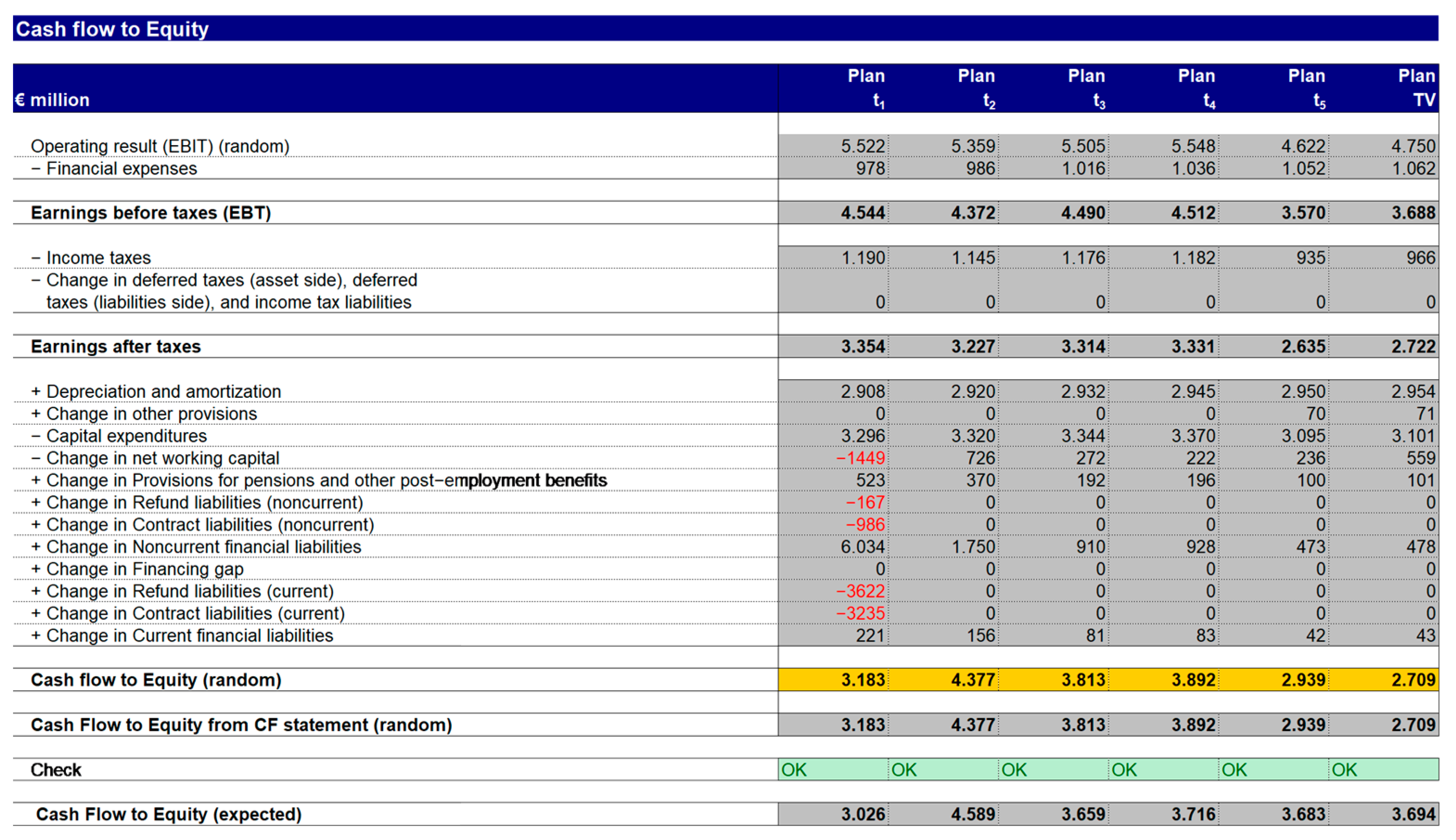
- Calculation of cash flows to equity as a target values of the Monte Carlo simulation.
- Risk analysis of the cash flows to equity.
- Pricing of the risk.
- Derivation of the cost of equity for the risk premium method.
- Calculation of the risk-adjusted cash flow to equity for the certainty equivalent method.
- Calculation of the company value with the risk premium method.
- Calculation of the company value with the certainty equivalent method.
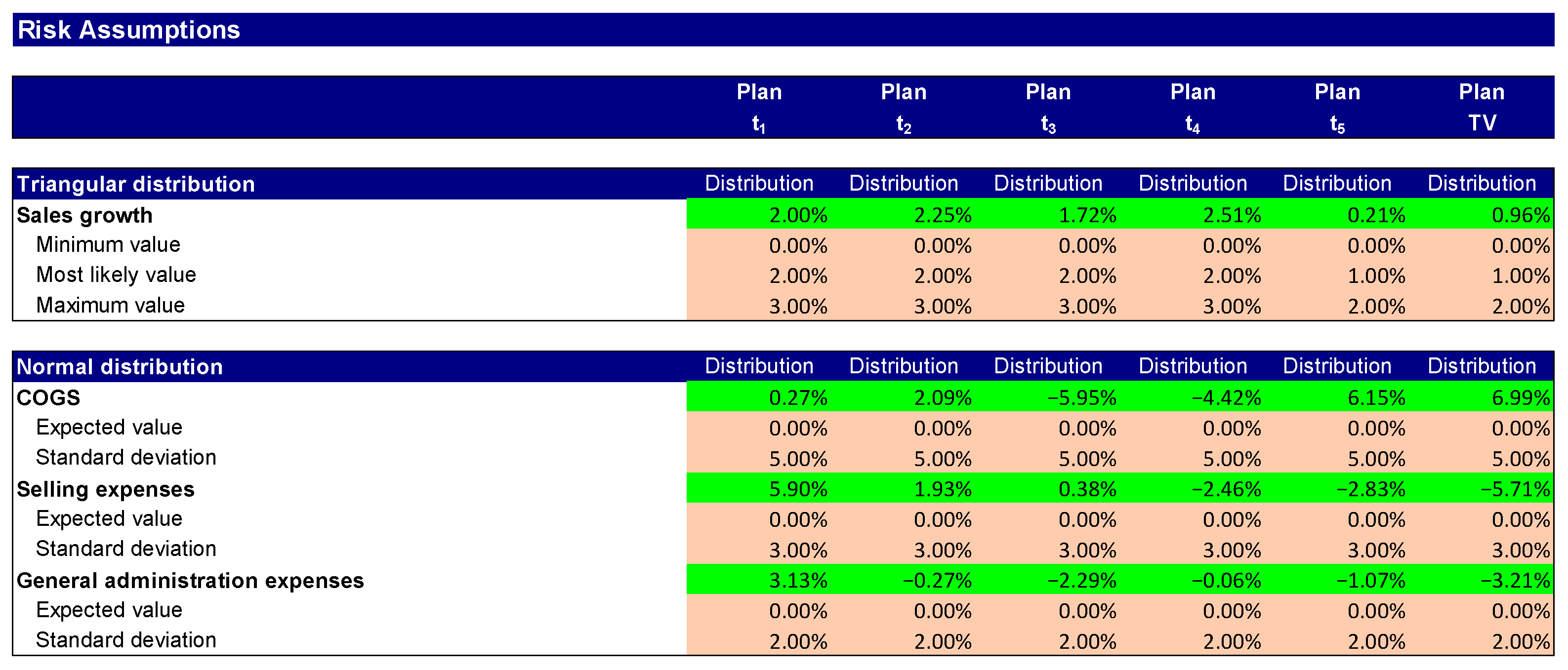
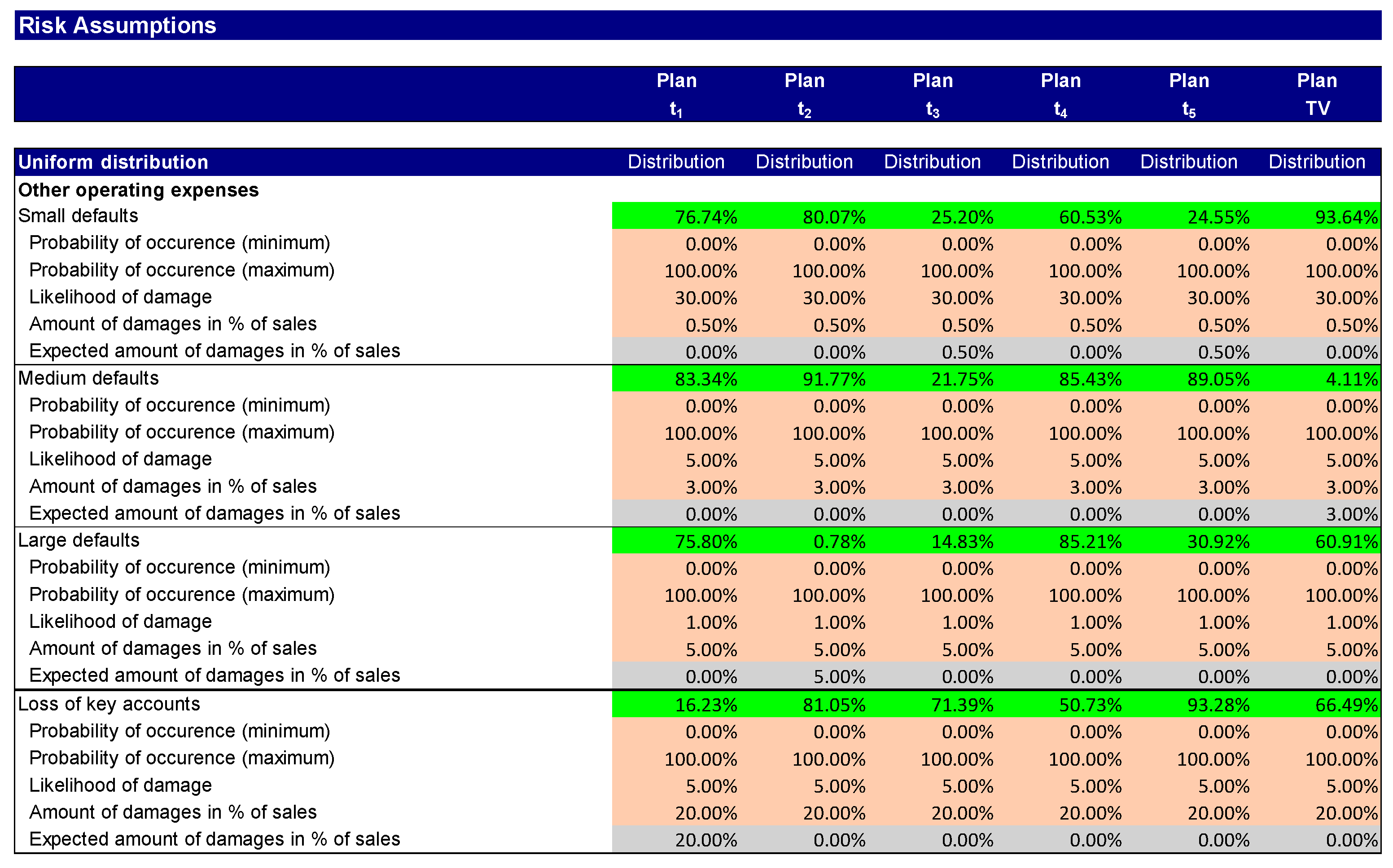
In step 1, as a result of a risk workshop, the risks that have not been hedged or can be hedged by the company are identified. These are quantified by assigning them a distribution function (Ernst and Wehrspohn 2022). Figure 1 shows the distribution functions for modelling total sales, COGS, and general administrative expenses. Figure 2 contains the distribution functions for modelling the other operating expenses. The cells with the green background colour are input cells for the Monte Carlo simulation and contain random numbers from the specified distribution functions.
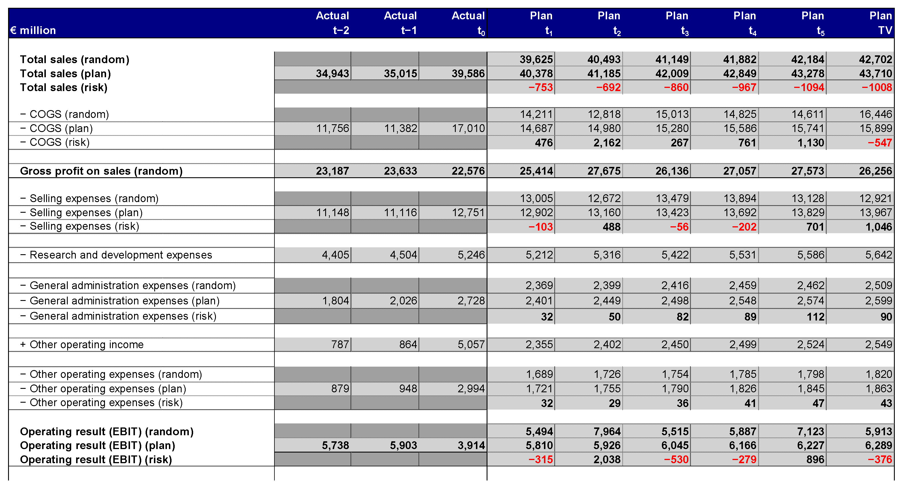
In the second step, the Monte Carlo parameters are built into the income statement and balance sheet planning. This results in unbiased planning. Figure 3 shows an excerpt of the income statement planning.
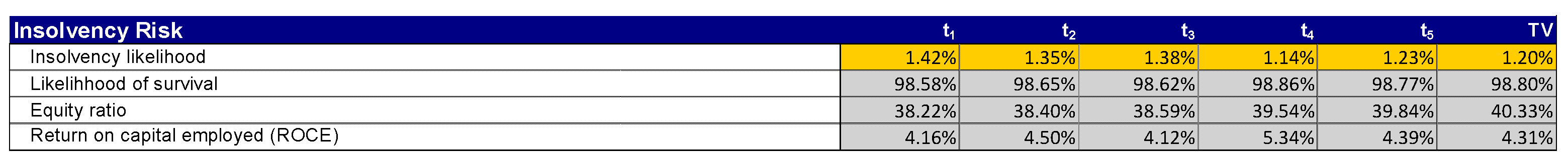
In step 3, the insolvency risk is linked to the planning model and the insolvency probability is calculated via a heuristic function using the equity ratio and the return on equity employed (ROCE) (see Figure 4). The cells with the yellow background colour are output cells of the Monte Carlo simulation.
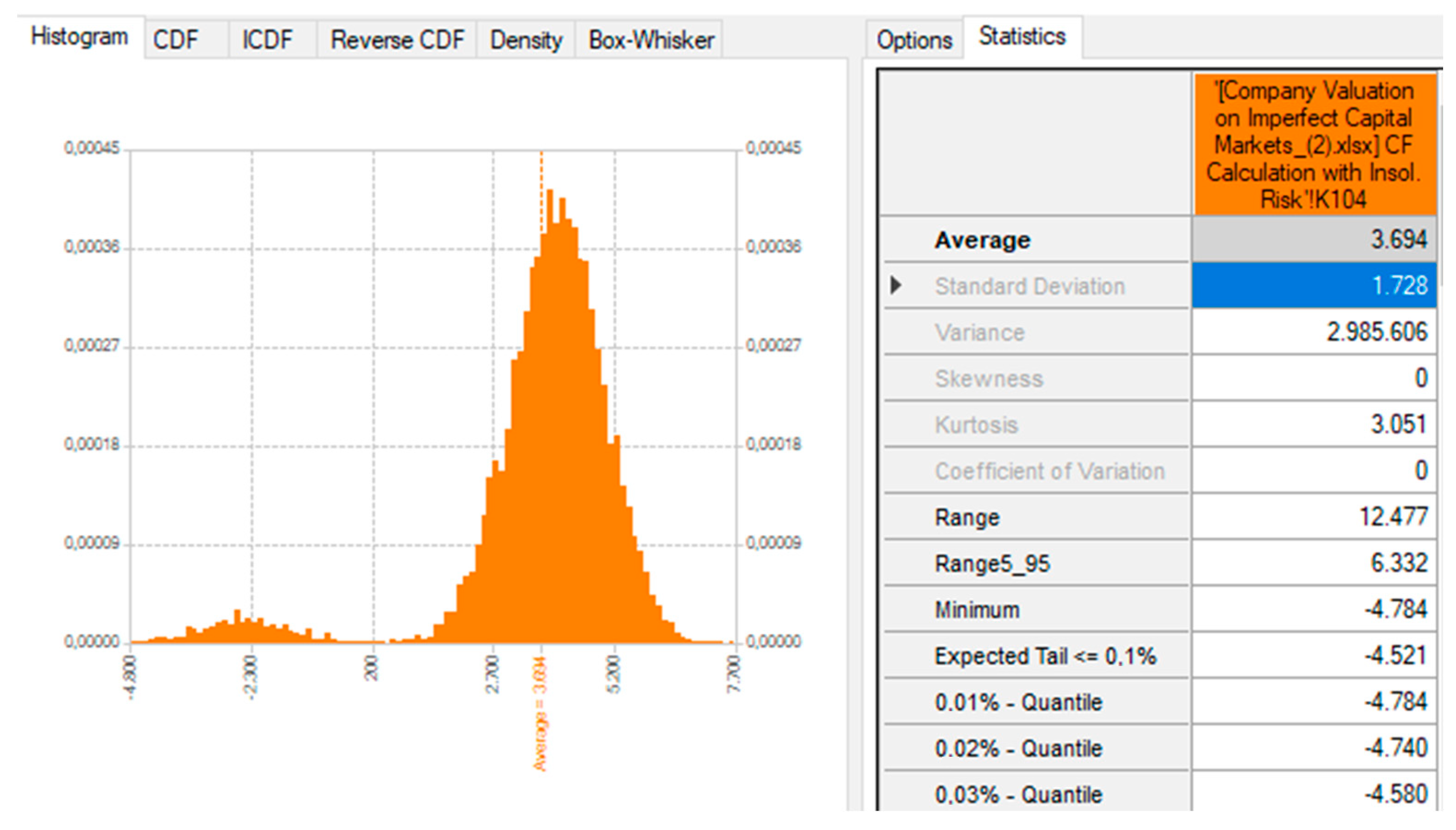
In step 4, the cash flows to equity are calculated as the target values of the Monte Carlo simulation (see Figure 5). The result of the Monte Carlo simulation is a frequency distribution of the cash flow to equity (see Figure 6), which is the basis for the following risk analysis. The tail risks in the frequency distribution are striking. They show that the combined occurrence of risks can threaten the existence of the company. These tail risks would be overlooked in the absence of simulation-based planning.
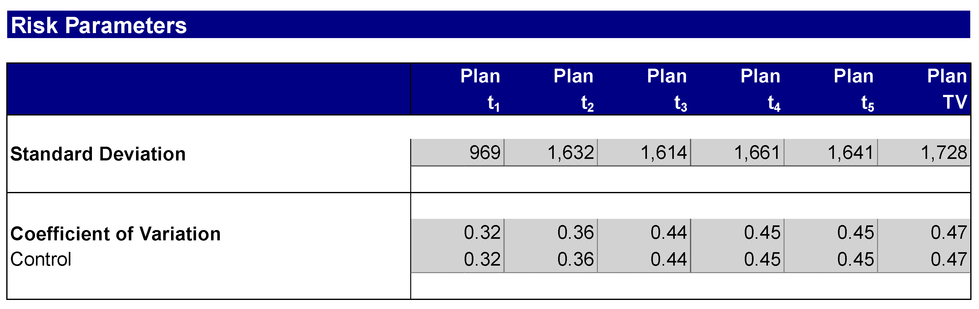
In step 5, the cash flow to equity risk analysis is carried out. The risk measures, standard deviation, and coefficient of variation are calculated (see Figure 7). The further calculations refer to the standard deviation for the certainty equivalent method and the coefficient of variation for the risk premium method.
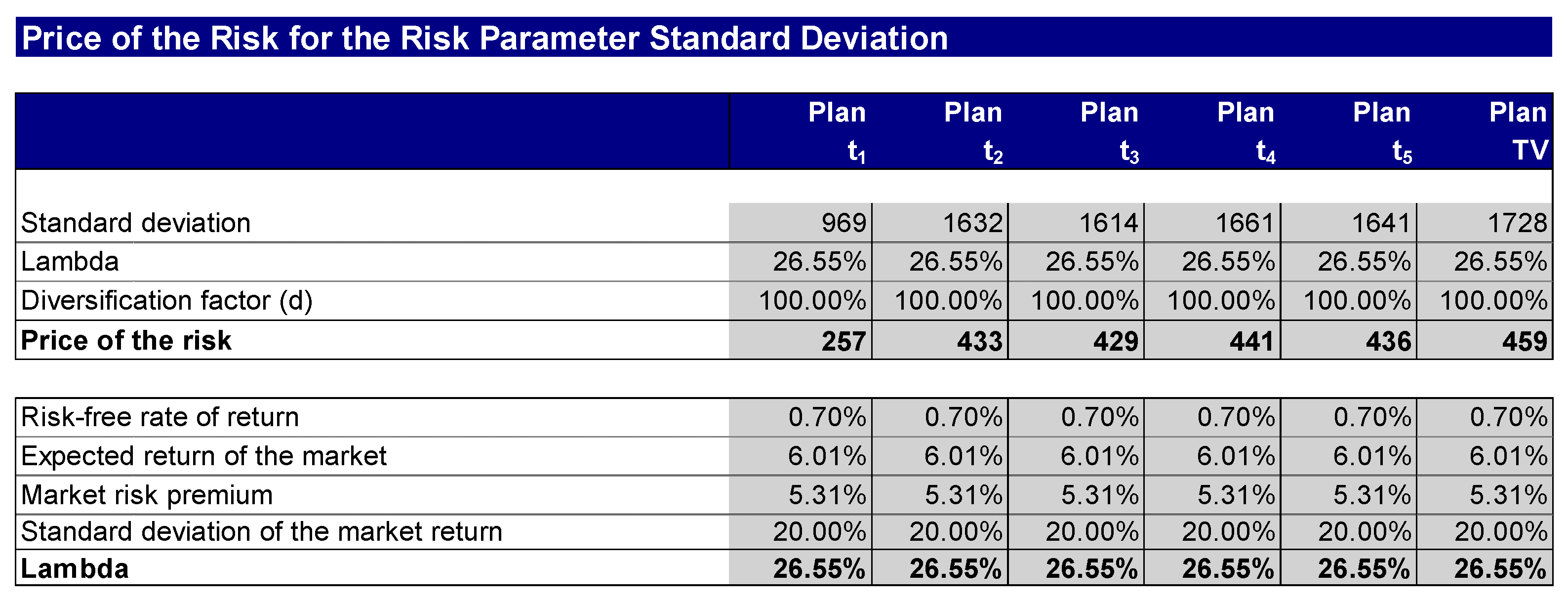
In step 6, the risk parameter—in our case the standard deviation—is adequately priced in order to determine risk-adjusted cash flows for the certainty equivalent method (see Figure 8). In addition to the risk parameter itself, this requires the market price of the risk and the diversification factor. The parameter lambda describes the “market price of the risk” and expresses the risk aversion. The lambda is calculated by setting the market risk premium in relation to one unit of market risk. The diversification factor depends on the investor’s diversification factor. In order to be able to take into account the entire risk scope of the company, the diversification factor is set at the value of one; however, the diversification factor can be adjusted individually.
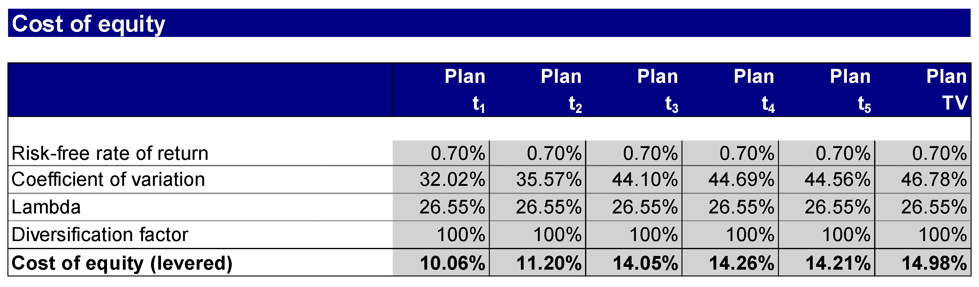
In step 7, the cost of capital for the risk premium method is derived from the certainty equivalents according to Equations (5) and (6). For the risk premium method, the risk is expressed in the cost of capital, in this case the cost of equity. The risk itself is the result of a risk analysis of the company, for which the coefficient of variation is calculated as the risk parameter. Figure 9 shows the cost of equity derived with the help of the coefficient of variation, the market price of the risk (lambda), and the diversification factor.
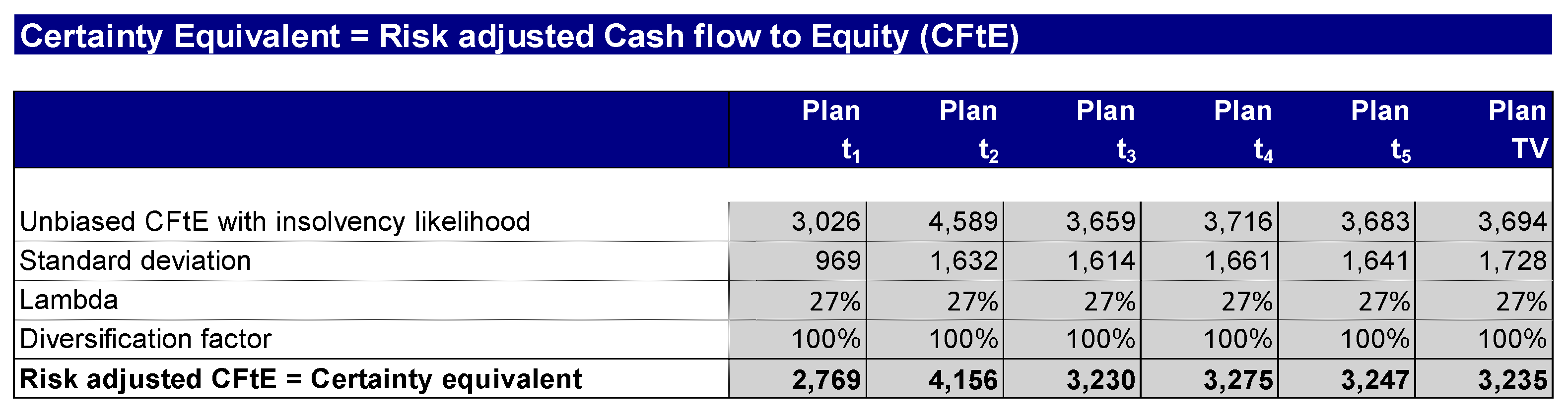
In step 8, the calculation of the risk-adjusted cash flow to equity for the certainty equivalent method, according to Equation (1), takes place. For the certainty equivalent method, the risk is calculated at the level of the cash flows. Figure 10 shows the risk-adjusted cash flows to equity underlying the valuation, which are also referred to as certainty equivalents.
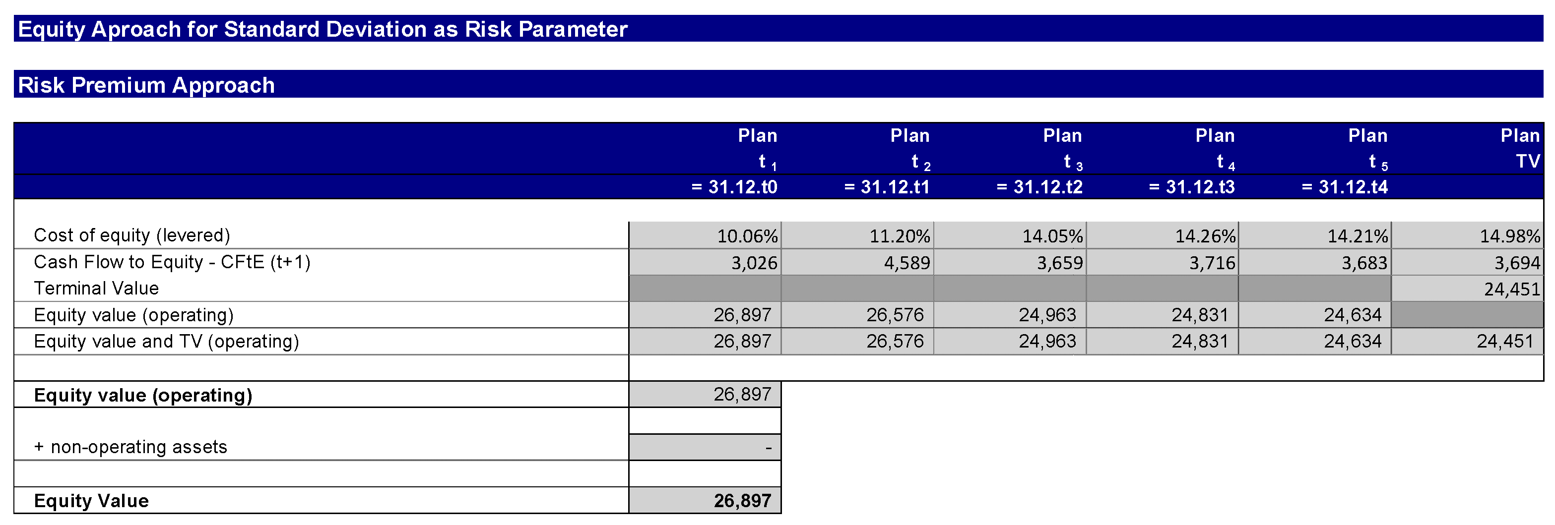
In step 9, the company value can be calculated retrogradely for the risk premium method starting from the terminal value (see Figure 11). The formulas derived above for the terminal value and the period-specific company value are used.
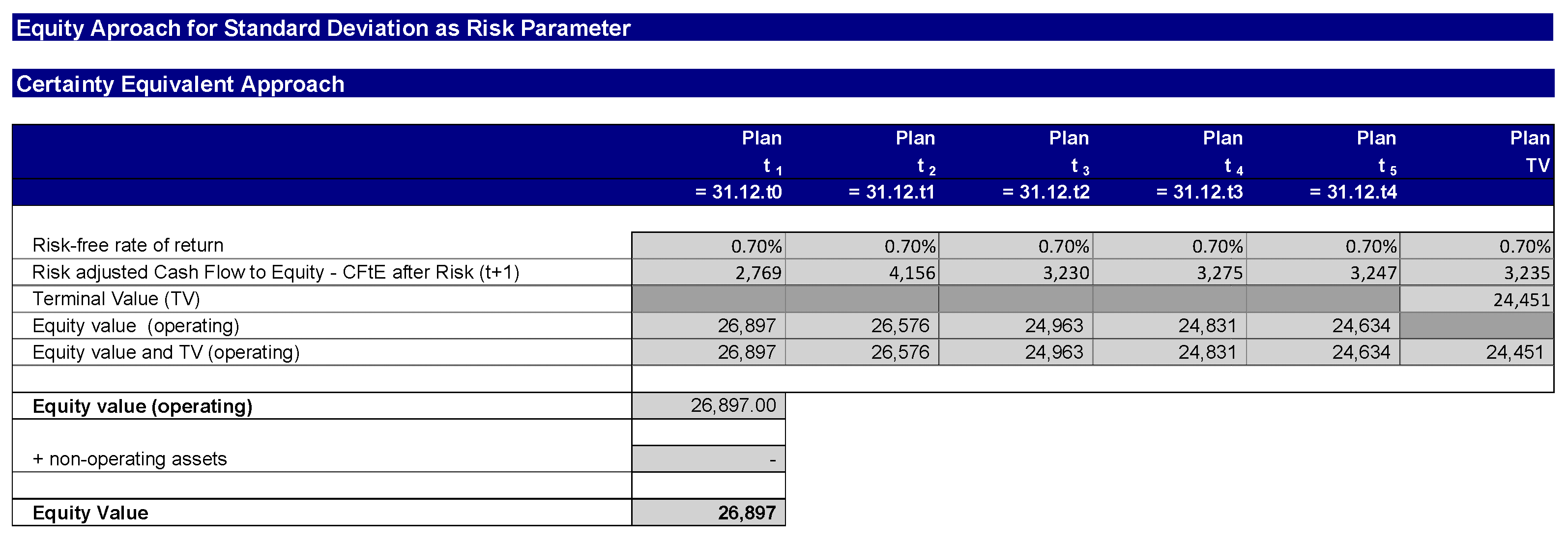
In step 10, the simulation-based business valuation for the certainty equivalent method is carried out (see Figure 12). Again, the formulas above are used.
It can be seen from the figures that the certainty equivalent method and the risk premium method lead to identical company values.
9. Results
Simulation-based business planning makes it possible to model imperfections in capital markets in the business valuation. This is done by means of unbiased planning that integrates the risks that are not hedged in the company into the business plan. Through a Monte Carlo simulation, the risks are aggregated to a target value (e.g., the cash flow). The frequency distribution of the cash flows serves as the basis for the company’s risk analysis. From this risk analysis, statements can be derived from risk ratios, the rating, the probability of insolvency, and the cost of capital.
The approach presented in this article makes it possible to supplement the CAPM-based DCF valuation that has, to date, predominated business valuation, with a DCF valuation that calculates risks not from the capital market, but from the risk potential that is actually present in the company.
The formulas presented in this article are intended to help valuation specialists familiar with CAPM-based DCF valuation to carry out a company valuation even when calculating the risk via the capital market does not seem sensible. The approach presented here makes it possible for valuation experts to transfer their valuation know-how to simulation-based business valuations, without having to overcome too many methodological hurdles. This is central for acceptance and application in valuation practice.
The approach presented here has limitations that require further research activities. The detailed planning period is well represented by the unbiased planning. The unbiased cash flows include the risks not hedged in the company and represent a suitable basis for valuation. Furthermore, the terminal value is based on a cash flow that is also unbiased and reflects the development associated with the risk, the probability of insolvency, and the growth in the continuation phase; however, the terminal value is based on the Gordon Growth formula, which is commonly used in practice. One area of research for the continuation phase would be to model the development of the cash flow via a stochastic process generated by a Monte Carlo simulation. This would have the advantage of applying a coherent approach to simulation-based planning and valuation for the entire planning horizon.
Another area of research is the determination of the diversification factor in simulation-based valuation. So far, CAPM-based company valuations assume a fully diversified investor. The counterpart to this is the total beta approach, which assumes an investor concentrated on one company. The degree of diversification depends on the individual asset situation of the investor; therefore, when determining the diversification factor, the investor’s overall asset situation must be determined. In order to be able to determine this, the Copula approach is required, which maps the correlation of the assets taking into account the correlations in the tails of the distribution functions of the assets. The connection of the Copula approach with simulation-based valuation is still an open area of research.
Since simulation-based planning and business valuation depicts the risks of many KPIs via frequency distributions, the fat tails of the distributions that can lead to risks, thus threatening the existence of the company, should be evaluated in particular. The extreme value theory can be used for this purpose.
Funding
The article processing charge was funded by the Baden-Württemberg Ministry of Science, Research and the Arts and Nürtingen-Geislingen University in the funding programme Open Access Publishing.
Institutional Review Board Statement
Not applicable.
Informed Consent Statement
Not applicable.
Data Availability Statement
Not applicable.
Conflicts of Interest
The author declares no conflict of interest.
References
- Brennan, Michael J., and Ashley W. Wang. 2010. The mispricing return premium. Review of Financial Studies 23: 3437–68. [Google Scholar] [CrossRef]
- Dempsey, Mike. 2013. The Capital Asset Pricing Model (CAPM): The History of a Failed Revolutionary Idea in Finance? Abacus 49: 7–23. [Google Scholar] [CrossRef]
- Dorfleitner, Gregor. 2020. On the use of the terminal-value approach in risk-value models. Annals of Operations Research, 1–21. Available online: https://epub.uni-regensburg.de/43131/1/Dorfleitner2020_Article_OnTheUseOfTheTerminal-valueApp.pdf (accessed on 22 February 2022). [CrossRef]
- Dorfleitner, Gregor, and Werner Gleißner. 2018. Valuing streams of risky cashflows with risk-value models. Journal of Risk 20: 1–27. [Google Scholar] [CrossRef]
- Ernst, Dietmar, and Joachim Häcker. 2017. Financial Modeling: An Introduction Guided to Excel and VBA Applications in Finance. London: Palgrave Macmillan. [Google Scholar]
- Ernst, Dietmar, and Joachim Häcker. 2021. Risikomanagement im Unternehmen. Bandar Seri Begawan: UTB. [Google Scholar]
- Ernst, Dietmar, and Uwe Wehrspohn. 2022. When Do I Take which Distribution? Berlin: Springer. [Google Scholar]
- Fama, Eugene F., and Kenneth R. French. 1993. Common risk factors in the returns on stocks and bonds. Journal of Financial Economics 33: 3–56. [Google Scholar] [CrossRef]
- Fama, Eugene F., and Kenneth R. French. 2008. Dissecting Anomalies. Journal of Finance 63: 1653–78. [Google Scholar] [CrossRef]
- Fama, Eugene F., and Kenneth R. French. 2012. Size, Value, and Momentum in international Stock Returns. Journal of Financial Economics 105: 457–72. [Google Scholar] [CrossRef]
- Fama, Eugene F., and Kenneth R. French. 2015. A five-factor asset pricing model. Journal of Financial Economics 116: 1–22. [Google Scholar] [CrossRef] [Green Version]
- Fishburn, Peter C. 1977. Mean-risk analysis with risk associated with below target returns. American Economic Review 67: 116–28. [Google Scholar]
- Gleißner, Werner. 2019. Cost of capital and probability of default in value-based risk management. Management Research Review 42: 1243–58. [Google Scholar] [CrossRef]
- Gleißner, Werner. 2020. Risikoanalyse und moderne Unternehmensbewertungsverfahren als Alternative zum CAPM. Controlling 32: 35–37. [Google Scholar] [CrossRef]
- Gleißner, Werner. 2021. Unternehmensbewertung: Methode und Nutzen. BewertungsPraktiker 3: 84–87. [Google Scholar]
- Gleißner, Werner, and Dietmar Ernst. 2019. Company valuation as result of risk analysis: Replication approach as an alternative to the CAPM. Business Valuation OIV Journal 1: 3–18. [Google Scholar] [CrossRef]
- Gordon, Myron. 1962. The Investment, Financing, and Valuation of the Corporation. Publisher Homewood, IL: Irwin. [Google Scholar]
- Haugen, Robert A. 2002. The Inefficient Stock Market: What Pays Off and Why. Hoboken: Prentice Hall. [Google Scholar]
- Hazen, Gordon. 2009. An extension of the internal rate of return to stochastic cashflows. Management Science 55: 1030–34. [Google Scholar] [CrossRef] [Green Version]
- Novy-Marx, Robert. 2013. The other side of value: The gross profitability premium. Journal of Financial Economics 108: 1–28. [Google Scholar] [CrossRef] [Green Version]
- Robichek, Alexander A., and Stewart C. Myers. 1966. Conceptual problems in the use of risk-adjusted discount rates. The Journal of Finance 21: 727–30. [Google Scholar]
- Rubinstein, Mark E. 1973. The Fundamental Theorem of Parameter Preference security valuation. Journal of Financial and Quantitative Analysis 8: 61–69. [Google Scholar] [CrossRef]
- Shiller, Robert J. 1981. The use of volatility measures in assessing market efficiency. Journal of Finance 36: 291–304. [Google Scholar] [CrossRef] [Green Version]
- Shleifer, Andrei. 2000. Inefficient Markets: An Introduction to Behavioral Finance. OUP Catalogue. Oxford: Oxford University Press. [Google Scholar]
- Smith, James E. 1998. Evaluating income streams:a decision analysis approach. Management Science 44: 1690–708. [Google Scholar] [CrossRef] [Green Version]
- Tversky, Amos, and Daniel Kahneman. 1979. Prospect theory: An analysis of decision under risk. Econometrica 47: 280–84. [Google Scholar] [CrossRef] [Green Version]
- Zhang, Chu. 2009. On the explanatory power of firm-specific variables in cross-sections of expected returns. Journal of Empirical Finance 16: 306–17. [Google Scholar] [CrossRef]
Figure 1.
Distribution functions for modelling total sales, COGS, and general administrative expenses.
Figure 1.
Distribution functions for modelling total sales, COGS, and general administrative expenses.

Figure 2.
Distribution functions for other operating expenses.

Figure 3.
Excerpt of the income statement planning.

Figure 4.
Insolvency risk.

Figure 5.
Calculation of the cash flow to equity.

Figure 6.
Frequency distribution and statics of the cashflow to equity in the TV.

Figure 7.
Calculation of the risk measures, standard deviation, and coefficient of variation.

Figure 8.
Pricing of the risk.

Figure 9.
Derivation of the cost of equity for the risk premium method.

Figure 10.
Calculation of the risk-adjusted cash flow to equity for the certainty equivalent method.
Figure 10.
Calculation of the risk-adjusted cash flow to equity for the certainty equivalent method.

Figure 11.
Calculation of the company value with the risk premium method.

Figure 12.
Calculation of the company value with the certainty equivalent method.

Publisher’s Note: MDPI stays neutral with regard to jurisdictional claims in published maps and institutional affiliations. |
© 2022 by the author. Licensee MDPI, Basel, Switzerland. This article is an open access article distributed under the terms and conditions of the Creative Commons Attribution (CC BY) license (https://creativecommons.org/licenses/by/4.0/).
Share and Cite
MDPI and ACS Style
Ernst, D. Simulation-Based Business Valuation: Methodical Implementation in the Valuation Practice. J. Risk Financial Manag. 2022, 15, 200. https://doi.org/10.3390/jrfm15050200
AMA Style
Ernst D. Simulation-Based Business Valuation: Methodical Implementation in the Valuation Practice. Journal of Risk and Financial Management. 2022; 15(5):200. https://doi.org/10.3390/jrfm15050200
Chicago/Turabian StyleErnst, Dietmar. 2022. "Simulation-Based Business Valuation: Methodical Implementation in the Valuation Practice" Journal of Risk and Financial Management 15, no. 5: 200. https://doi.org/10.3390/jrfm15050200